Coursera - Data Engineering with GCP

Course 1 - Google Cloud Platform Big Data and Machine Learning Fundamentals

According to McKinsey - by 2020 there will be 5bln connected devices, with amount of data doubling every two years. Also it is estimated that only 1% of this data is currently analyzed.

Big Data Challenges are:

Migrating existing data workloads (ex. Hadoop, Spark)
Analyzing large datasets at scale (note “large” means Tbs or Pbs)
Building scalable streaming data pipelines
Applying machine learning models to your data

Course 1.1 - Introduction to GCP

Introduction to GCP which is behind 7 cloud products with 1bn monthly users. And GCP itself is responsible for hosting another ~1bn of end-users with GCP customer products.

Three key layers:

base layer is Security
2nd layer is Compute, Storage and Networking
3rd layer is Big Data and ML products to abstract away the BD and ML infrastructure

Compute

From 2018 estimates, roughly 1.2 billion photos and videos are uploaded to the Google Photos service everyday. That is 13 plus petabytes of photo data in total. For Youtube - 60Pb of data every hour.

Moore’s law is not valid since ~2003-2005, now the compute power doubles only every ~20yrs or so. One solution is ASIC, and Google’s Tensor Processing Unit is one of the examples of ASIC. TPUs brought 10x increase in ML training/iterations of models.

GCP demo covering:

creating and preparing compute VM
creating bucket
copying processed data to the bucket and stopping VM
changing permissions of files in the bucket to public
viewing static site on storage.googleapis

Storage

Four classes of storage:

Multi-regional
Regional
Nearline
Coldline

Resource hierarchy:

Resources
Projects, provide logic grouping of resources
Folders, can combine projects
Organization, group node for the enterprise-level of policies

Networking

Google private network connecting GCP data centers carries ~40% of entire internet traffic. Fast network allows separating computations and data across multiple data centers w/o compromising communications between resources.

Security

The last piece of basic insfrastructure. In the on-premise deployments you are responsible for security across all layers, including networking, hardware, storage, deployment, etc. As you move towards managed services you can offload these concerns to GCP, so you are left with security on Content, Access Policies and Usage.

In-transit encryption, encryption at rest and distributed for access/storage. BigQuery security controls as an example.

Evolution of GCP

2002 - Google File System
2004 - MapReduce, which led to Hadoop
2006 - YouTube and high data volume led to BigTable, which inspired other no-sql databases
2008 - Dremel as a substitution of MapReduce
2013 - PubSub and DataFlow
2015 - Tensorflow
2017 - TPUs
2018 - AutoML

Choosing the right approach/product. Starting from IaaS in terms of Compute, GKE, App Engine as PaaS and Cloud Functions and FaaS.

Key roles in Big Data companies:

Data Engineers to build pipelines
Decision Makers for investment
Data Analysts to explore data for insights
Statisticians
Applied ML Engineers
Data Scientists
Analytics Managers

Course 1.2 - Recommending System using Spark and Cloud SQL

Product Recommendations is one of the most common business tasks. Example of application - housing recommendation system on premise. Data is stored in Hadoop. There is an ML model running as SparkML job on data in Hadoop daily with results of the recommendation stored in MySQL. This is all running on premise. Now we are interested in moving to GCP. We’ll move the SparkML job as DataProc with results stored in Cloud SQL.

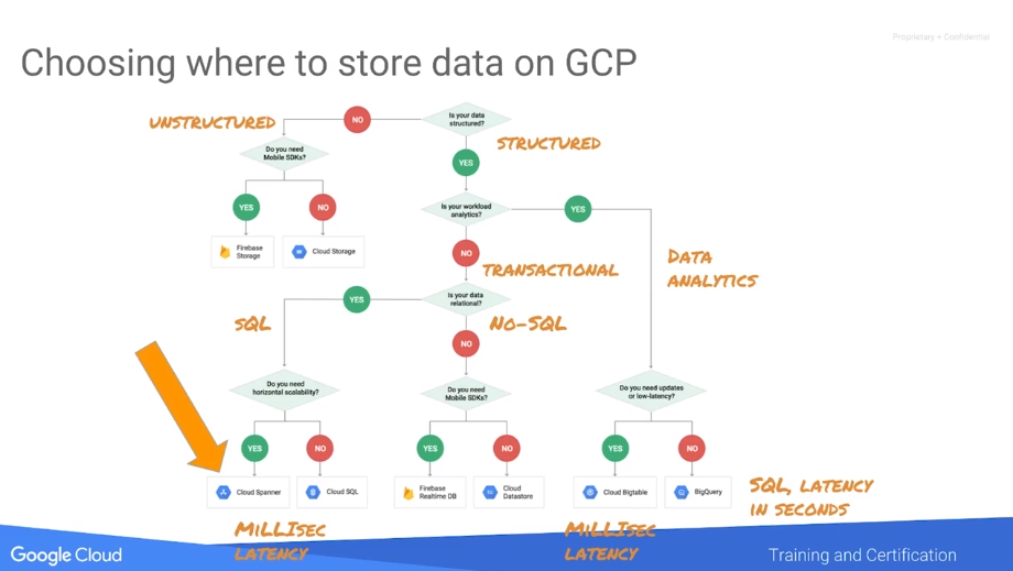
Typical patterns for choosing the right database solution:

“Cloud Storage” for blob file storage
“Cloud SQL” for gigabytes-level SQL storage on the cloud. If data > Gbs and > 1 table -> “Cloud Spanner”
“Cloud Datastore” for structured data from App Engine, transactional no-SQL.
“BigTable” for non-transactional, high throughput flat data (sensors)
“BigQuery” for data warehousing

Cloud Dataproc provides a managed service for creating Hadoop and Spark clusters, and managing data processing workloads.

Open-source ecosystem running on Hadoop:

Hadoop is canonical MapReduce framework
Pig is a scripting language to create MapReduce jobs
Hive is data warehousing system
Spark is a fast interactive general-purpose framework to run analytics, leveraging in-memory processing

Demo starting a Spark job on Hadoop cluster using DataProc in less than 10min.

Lab covering the following:

Creating Cloud SQL cluster and database with three tables
Importing data to Cloud SQL from buckets and running queries
Creating DataProc cluster
Submitting a PySpark job running on Cloud SQL cluster

Course 1.3 - Predict visitor purchases with BigQuery ML

BigQuery as a petabyte-scale analytics warehouse. BQ is actuall two services: a fast SQL Query Engine and fully managed data storage.

BQ features:

Serverless
Flexible pricing
Data encryption and security
Geospatial data types
Foundation for BI and AI

Typical BQ solution architecture: batch (cloud storage) and streaming (pub/sub) pipelines feeding the BQ via Dataflow. BQ can then expose data through DataStudio, Tableau, Qlik, Looker and even Google spreadsheets.

Demo of querying github 2M repos dataset to determine tabs vs spaces ratio by programming language. One SQL script, executed over 155Gb of data in 13sec with ~50min of actual nodes work time.

BQ storage hierarchy is Datasets consisting zero or more tables, each consisting columns. Columns are compressed and stored in Colossus filesystem.

Demo of exploring public bike share dataset in SFO area with just SQL. CREATE or REPLACE to store results in a table or a view, which provides logic only.

Misc quick notes:

Cloud Dataprep (partnership with Trifecta) to provide visualizations to evaluate the quality of data in BQ.
Scheduling BQ SQL jobs with @run_time
Use BQ queries on federated data sources (GCS, Google drive, CSV)
Streaming data into BQ through API or DataFlow
BQ natively supports structs and arrays for the case of data normalization
BQ natively supports GIS, BQ Geo Viz also gives a free GIS visualization tool

BigQuery ML

Simple decision tree for choosing the right ML models:

Linear regression for time-series forecast
Logistic regression (single or multi-class) for classification
Matrix factorization for recommendation
Clustering for unsupervised

Built-in functions for training and prediction inside SQL. BQ ML supports basic features, such as auto-tuning learning rate and auto-splitting into training and test datasets, but also supports more advanced like regularization, different training/test splits, custom learning rates, etc. Supports linear regression and logistic regressions. Supports different metrics, inspecting weights, etc.

E2E BQML process:

ETL data into BQ
Preprocess features
Create model
Evaluate model
Use model for predictions

Alias a label column as label or specify it in options.

Lab on BQ ML

Example of model creation based on Google Analytics dataset with two features and one label:

CREATE OR REPLACE MODEL `ecommerce.classification_model`
OPTIONS
(
model_type='logistic_reg',
labels = ['will_buy_on_return_visit']
)
AS

#standardSQL
SELECT
  * EXCEPT(fullVisitorId)
FROM

  # features
  (SELECT
    fullVisitorId,
    IFNULL(totals.bounces, 0) AS bounces,
    IFNULL(totals.timeOnSite, 0) AS time_on_site
  FROM
    `data-to-insights.ecommerce.web_analytics`
  WHERE
    totals.newVisits = 1
    AND date BETWEEN '20160801' AND '20170430') # train on first 9 months
  JOIN
  (SELECT
    fullvisitorid,
    IF(COUNTIF(totals.transactions > 0 AND totals.newVisits IS NULL) > 0, 1, 0) AS will_buy_on_return_visit
  FROM
      `data-to-insights.ecommerce.web_analytics`
  GROUP BY fullvisitorid)
  USING (fullVisitorId)
;

</Lab>

Course 1.4 - Create Streaming Data Pipelines with Cloud Pub/sub and Cloud Dataflow

First challenge - handling large volumes of streaming data, not coming from the single source. Solution is - Cloud Pub/Sub.

Cloud Pub/Sub:

at-least-once delivery
exactly-once processing
no provisioning
open APIs
global by default
e2e encryption

Common architecture is: Ingest -> Cloud Pub/Sub for storing -> Dataflow for processing -> BQ or SQL for Storing and Analyzing -> Explore and Visualize

During streaming pipelines design the Data Engineer needs to address two questions:

Pipeline design (Apache Beam)
Pipeline implementation (Dataflow)

Apache Beam is Unified, Portable, Extensible. Has a syntax very similar to scikit-learn pipelines. You can write a code in Java, Go, python and deploy in Runner (Spark, Dataflow). Dataflow is scalable, serverless and has Stackdriver integrated in it. After deploying a pipeline in Dataflow it will automatically optimize it, scale up workers, heal workers, connect to many different sinks.

DataStudio can work with multiple datasources. Some ramifications - anyone who can see the dashboard can potentially see the whole datasources. Anyone who can edit the dashboard can see all fields.

Some dashboard tips:

start with KPIs at the top
below have sections with details, starting with the question “What are the sales channels?” to grab user attention
you can fix time filters to some specific periods

Lab Lab on setting up a Dataflow pipeline connecting to the public pub/sub topic on NY taxi rides, outputting the results to BQ. Creating a SQL query on BQ to output the summary of rides with passengers, rides and total revenue. Connecting Datastudio for creation of the streaming dashboard. </Lab>

Course 1.5 - Classify Images with Pre-Built Models using Vision API and Cloud AutoML

Examples of business applications:

pricing cars based on images
NPL to route emails to correct support
image recognition to mark inappropriate content in images
Dialogflor for new shopping experience
predicting empty or full cargo ships based on the satellite image

Approaches to ML according to GCP:

Pre-Built AI products
Custom models on top of AutoML
New models entirely with training

Vision API: cloud.google.com/vision

By 2021 enterpises will use 50% more chatbots - GCP Dialogflow.

Text classification problem done in three ways using GCP

Predicting which publication the article came from, based on just 5 first letters in the title.

BQ ML: sql processing to create training dataset. Use BQ ML to train, evaluate and predict
AutoML Natural Language: takes few hours to train
Custom model using ML Engine Jupyter notebooks. Jupyter magic to use BQ inside notebooks.

Course 2 - Leveraging Unstructured Data

Unstructured data is seen as “digital exhaust”. Big, expensive to process.

Course 2.1 - Introduction to Dataproc

Data you collect, but don’t analyze, because it is too hard, usually. This is the data, which can be described by 3Vs: veracity, velocity, and volume.

Structured data has schema. Unstructured data is a relative term. It may have schema, but not suitable for analysis. About 90% of enterprise data is unstructured.

Dataproc is GCP implementation of Hadoop.

Horizontal scaling (cloud) vs vertical scaling (mainframe).

In early 2000 Google realized the need to index all web. In 2004 Google proposed MapReduce. Map splits BigData and maps it to some structure and Reduce reduces to some meaningful results. Later the Google File System was created to manage distributed storage. Apache developed an OSS alternative, called Hadoop, with Hadoop File System. Pig, Hive and Spark are parts of the ecosystem built on top of Hadoop.

Apache Spark is an important innovation, which allows managing multiple various workflows (say sensor processing vs image processing) and map it to available Hadoop resources. Spark follows the Declarative paradigm, i.e. it decides how to do things, based on What you want.

… marketing speech on why GCP is better than on-premise cluster …

Options for creating Hadoop cluster:

on-premise
vendor-managed
bdutil (OSS utility to create clusters using VMs) - DEPRECATED in favor of Dataproc
Dataproc

Dataproc on average takes 90sec to provision from start to beginning of processing.

Dataproc customization:

single node cluster (good for experimentation)
standard (one master node)
high-availability (three master nodes)

Don’t use HDFS for cloud storage. Dataproc cluster should be stateless, so you can turn it on/off as needed.

Lab - Creating Hadoop cluster and exploring it

Create a VM to control the cluster. SSH into a vm. Setup environment variables (not sure why, as all provisioning was done in WebUI). Setup and start the 3-worker node cluster. Create firewall rule using a network tag. Make sure that cluster master has a right network tag. Connect to its public IP to see Hadoop cluster status. </Lab>

Choosing the right size of your VMs

Pick the number of vCPUs and RAM to match the job requirements. GCP WebUI allows to copy/paste the custom code for the customized VM.

Preemptible VMs are up to 80% cheaper than standard. Use PVMs only for processing. Use it for non-critical processing and in large clusters. Rule of thumb - anything over 50/50 ratio of PVMs vs standard may have diminishing returns. Dataproc manages adding and removing PVMs automatically.

Course 2.2 - Running Dataproc jobs

Dataproc includes some of the most common Hadoop frameworks: Hive, Pig and Spark. Hive is declarative, Pig is imperative.

Lab - Hive and Pig jobs

Example of Pig job:

rmf /GroupedByType
x1 = load '/pet-details' using PigStorage(',') as (Type:chararray,Name:chararray,Breed:chararray,Color:chararray,Weight:int);
x2 = filter x1 by Type != 'Type';
x3 = foreach x2 generate Type, Name, Breed, Color, Weight, Weight / 2.24 as Kilos:float;
x4 = filter x3 by LOWER(Color) == 'black' or LOWER(Color) == 'white';
x5 = group x4 by Type;
store x5 into '/GroupedByType';

Pig provides SQL primitives similar to Hive, but in a more flexible scripting language format. Pig can also deal with semi-structured data, such as data having partial schemas, or for which the schema is not yet known. For this reason it is sometimes used for Extract Transform Load (ETL). It generates Java MapReduce jobs. Pig is not designed to deal with unstructured data.

</Lab>

Bring the data to compute - vertical scaling. As we moved to the distributed computing one approach was to keep data local to machines in the cluster. However given the MTBF of modern drives the reliability of such approach is quite low. In 2002 Google introduced Google File System to introduce redundant file system.

In 2006 Google develops BigTable and BQ Query Language. Colossus is around same time and is a replacement of GFS and is foundation of Cloud Storage.

Nowadays GCP has a mix of PC or cluster-based products (Dataproc), managed services (Cloud SQL) and completely serverless abstract services (BQ, Dataflow, ML products, etc).

If you look at replacing the on-premise ETL pipeline with GCP it will roughly consist of:

Pub/Sub for Ingest
Dataflow for Processing
BigQuery for Analysis

Networking

In distributed architecture networking has to manage horizontal (East-West) communications vs vertical (South-North) in case of traditional client-server applications. With petabyte bisectional bandwidth the data may be stored separately from compute.

Submitting Spark jobs

Spark jobs can be submitted from master node, but the preferred method is to submit from cluster console or gcloud console.

Easiest way to migrate:

Copy data to GCP Cloud Storage
Update file links from hdfs to gs://
Upload Spark jobs

Spark uses RDD and manages all infrastructure. Spark has Lazy evaluation and uses DAGs to store jobs. And it chooses the most effective way to organize and implement jobs, given other jobs and available resources.

Lab - Submit Dataproc jobs for unstructured data v1.3

Create dataproc, explore pyspark in interactive commands. Create and submit a job to process two text files:

from pyspark.sql import SparkSession
from operator import add
import re

print("Okay Google.")

spark = SparkSession\
        .builder\
        .appName("CountUniqueWords")\
        .getOrCreate()

lines = spark.read.text("/sampledata/road-not-taken.txt").rdd.map(lambda x: x[0])
counts = lines.flatMap(lambda x: x.split(' ')) \
                  .filter(lambda x: re.sub('[^a-zA-Z]+', '', x)) \
                  .filter(lambda x: len(x)>1 ) \
                  .map(lambda x: x.upper()) \
                  .map(lambda x: (x, 1)) \
                  .reduceByKey(add) \
                  .sortByKey()
output = counts.collect()
for (word, count) in output:
  print("%s = %i" % (word, count))

spark.stop()

</Lab>

TL;DR: We explored three intefaces to submit Dataproc jobs - Hive, Pig and Spark.

Leveraging GCP when working with Dataproc - BigQuery and Cluster Optimization

Dataproc cannot work directly with BQ, but we can use GCS as an intermediary to connect the two. One option is to export data from BQ in shards to GCS, so Dataproc can consume it from there. Symmetrically Dataproc can export data to GCS, which can be imported to BQ. Second options is to use the PySpark connector to BigQuery. You cannot run a query inside the connector, so you should run a query in BQ, export it and then import to RDD.

One more option is to use Pandas. Pandas can read from BQ and Dataproc (pyspark) can work with pandas. Pandas dataframe (easy to use, mutable) can be converted into Spark dataframe (faster, immutable).

Lab - Leverage GCP Explore Spark using PySpark jobs, use Cloud Storage instead of HDFS, and run a PySpark application from Cloud Storage.

Same as previous lab, except:

files are served from GCS
job was submitted via pyspark and also via Dataproc job interface in GCP

</Lab>

Dataproc can read and write to: BigTable, BigQuery, CloudStorage, etc.

You can also install various OSS frameworks on Dataproc clusters (e.g. Kafka). Installation scripts can help with installing OSS on master or worker nodes (e.g. Cloud Datalab). You need to create a script (bash, python), upload to GCS and specify location during Dataproc creation.

Lab - Cluster automation using CLI commands In this lab, you will create a cluster using CLI commands and learn about the Dataproc-GCP workflow and workflow automation.

Steps:

SSH to compute VM
clone training repository, update init-script to install python and clone repo to all nodes
create Dataproc cluster with two custom init-scripts, see below
wait for creation and validate Datalab installation

gcloud dataproc clusters create cluster-custom \
--bucket $BUCKET \
--subnet default \
--zone $MYZONE \
--region $MYREGION \
--master-machine-type n1-standard-2 \
--master-boot-disk-size 100 \
--num-workers 2 \
--worker-machine-type n1-standard-1 \
--worker-boot-disk-size 50 \
--num-preemptible-workers 2 \
--image-version 1.2 \
--scopes 'https://www.googleapis.com/auth/cloud-platform' \
--tags customaccess \
--project $PROJECT_ID \
--initialization-actions 'gs://'$BUCKET'/init-script.sh','gs://cloud-training-demos/dataproc/datalab.sh'

Creating firewall rule for Dataproc

gcloud compute \
--project=$PROJECT_ID \
firewall-rules create allow-custom \
--direction=INGRESS \
--priority=1000 \
--network=default \
--action=ALLOW \
--rules=tcp:9870,tcp:8088,tcp:8080 \
--source-ranges=$BROWSER_IP/32 \
--target-tags=customaccess

</Lab>

Lab - Leveraging ML

Three pyspark jobs using NLP ML APIs:

#!/usr/bin/env python
# Copyright 2018 Google Inc.
#
# Licensed under the Apache License, Version 2.0 (the "License");
# you may not use this file except in compliance with the License.
# You may obtain a copy of the License at
#
#     http://www.apache.org/licenses/LICENSE-2.0
#
# Unless required by applicable law or agreed to in writing, software
# distributed under the License is distributed on an "AS IS" BASIS,
# WITHOUT WARRANTIES OR CONDITIONS OF ANY KIND, either express or implied.
# See the License for the specific language governing permissions and
# limitations under the License.

'''
  This program takes a sample text line of text and passes to a Natural Language Processing
  services, sentiment analysis, and processes the results in Python.
  
'''

import logging
import argparse
import json

import os
from googleapiclient.discovery import build

from pyspark import SparkContext
sc = SparkContext("local", "Simple App")

'''
You must set these values for the job to run.
'''
APIKEY="AIzaSyDqqwkFJ3y7tGnBKXM4eFFAoLWpWtdLXCk"   # CHANGE
print(APIKEY)
PROJECT_ID="qwiklabs-gcp-00-621c25f27aea"  # CHANGE
print(PROJECT_ID) 
BUCKET="qwiklabs-gcp-00-621c25f27aea"   # CHANGE


## Wrappers around the NLP REST interface

def SentimentAnalysis(text):
    from googleapiclient.discovery import build
    lservice = build('language', 'v1beta1', developerKey=APIKEY)

    response = lservice.documents().analyzeSentiment(
        body={
            'document': {
                'type': 'PLAIN_TEXT',
                'content': text
            }
        }).execute()
    
    return response

## main

sampleline = 'There are places I remember, all my life though some have changed.'
#

# Calling the Natural Language Processing REST interface
#
results = SentimentAnalysis(sampleline)

# 
#  What is the service returning?
#
print("Function returns: ", type(results))

print(json.dumps(results, sort_keys=True, indent=4))

</Lab>

Course 3 - Serverless Data Analysis

BigQuery is No-Ops Data Warehousing and Analytics. Dataflow is No-Ops Data pipelines for reliable, scalable data processing.

Course 3.1 - BigQuery

BQ is a part of 2nd generation of Big Data at Google. Dataproc is 1st generation. BQ is beginning of Gen2, done in 2006, Dataflow is from 2014. MapReduce is Gen1 and it had a preliminary step of splitting data into shards in Map step, this is not scaling well, however. Dremel is an internal version of BigQuery, used at Google.

Hierarchy (top to bottom):

Project (billing info, users)
Dataset (organization, access control on dataset basis)
Table (data with schema, you join tables in dataset)

Job stores queries, handles export and copy.

Dataset contains Tables and Views. View is a live view of the Table (it is a query underneath), you can use View to manage access control through “SELECT” and filtering what you want to show. Views are virtual Tables. BigQuery engine can work both with BQ Tables and external sources of information. Job can take seconds to hours, you get charged based on the compute resources used to process the query.

BigQuery storage is columnar, every column is stored in a separate, encrypted, compressed file, replicated 3 times. No indexes, keys. One way to optimize queries is to filter out columns you run the query against.

BQ SQL tips:

BQ Query language is 2011 + extensions.
Format of table in FROM is <project>.<dataset>.<table>. If you leave out project it will be the current project by default.
You can embed the one query in another as a table and include it in FROM field.
Can select from multiple tables, joined by coma
Can JOIN ON field across tables inside the query
Reminder that GROUP requires aggregation function in SELECT

Lab 1 - Building BQ Queries

Examples of queries demonstrating various solutions are below.

SELECT
  f.airline,
  COUNT(f.departure_delay) AS total_flights,
  SUM(IF(f.departure_delay > 0, 1, 0)) AS num_delayed
FROM
   `bigquery-samples.airline_ontime_data.flights` AS f
WHERE
  f.departure_airport = 'LGA' AND f.date = '2008-05-13'
GROUP BY
  f.airline

Selecting all rainy days for given weather station and joining it on date with flights table.

SELECT
  f.airline,
  SUM(IF(f.arrival_delay > 0, 1, 0)) AS num_delayed,
  COUNT(f.arrival_delay) AS total_flights
FROM
  `bigquery-samples.airline_ontime_data.flights` AS f
JOIN (
  SELECT
    CONCAT(CAST(year AS STRING), '-', LPAD(CAST(month AS STRING),2,'0'), '-', LPAD(CAST(day AS STRING),2,'0')) AS rainyday
  FROM
    `bigquery-samples.weather_geo.gsod`
  WHERE
    station_number = 725030
    AND total_precipitation > 0) AS w
ON
  w.rainyday = f.date
WHERE f.arrival_airport = 'LGA'
GROUP BY f.airline

</Lab>

Loading and Exporting Data to BigQuery

Data may arrive from multiple different ingestions and capturing services. It will goes through processing service, such as Dataproc or Dataflow. Dataflow can treat both batch and streaming data. It will get stored either in objects in Cloud Storage or in tables in BigQuery storage. For analysis it may go through BigQuery Analytics service (SQL). And eventually it will end in either one of 3rd party services or in DataStudio.

You can also load data into BigQuery using CLI, WebUI, API

Lab 2 - Loading and Exporting data

Loading data from cloud shell.

bq load --source_format=NEWLINE_DELIMITED_JSON $DEVSHELL_PROJECT_ID:cpb101_flight_data.flights_2014 gs://cloud-training/CPB200/BQ/lab4/domestic_2014_flights_*.json ./schema_flight_performance.json.dumps

Exporting to gcs bucket:

bq extract cpb101_flight_data.AIRPORTS gs://$BUCKET/bq/airports2.csv

</Lab>

Advanced Capabilities in BigQuery

BQ supports all standard SQL data types. WITH statement allows to use subqueries before SELECT. COUNT(DISTINCT) function.

Normalization Normalizing the data means turning it into a relational system. This stores the data efficiently and makes query processing a clear and direct task. Normalizing increases the orderliness of the data. Denormalizing is the strategy of accepting repeated fields in the data to gain processing performance. Data must be normalized before it can be denormalized. Denormalization is another increase in the orderliness of the data. Because of the repeated fields, in the example, the Name field is repeated, the denormalized form takes more storage. However, because it no longer is relational, queries can be processed more efficiently and in parallel using columnar processing.

Nested columns can be understood as a form of repeated field. It preserves the relationalism of the original data and schema while enabling columnar and parallel processing of repeated nested fields. Nested and repeated fields helps BigQuery more easily interact with existing databases enabling easier transitions to BigQuery and hybrid solutions where BigQuery is used in conjunction with traditional databases.

Performance and Pricing

Less work -> Faster query Work:

I/O
Shuffle - how many bytes are passed to next stage
Grouping - how much is passed to every group
Materialization - how many bytes did you write
CPU - number and complexity of UDFs

Tips:

Don’t project unnecessary columns.
Filter and do WHERE as early as possible
Do biggest JOINs first, filter before JOINs
When you do GROUPing, consider how many rows are passed. Low cardinality keys/groups - faster
High cardinality may also lead to long tailing, shuffling and lots of groups with only 1 member
Built-in functions are more effective than SQL UDFs and even more than Javascript UDFs
Check if there is an approximate built-in function close to what you expect
ORDER goes on the outermost query
Use wildcards in table names.
Partition table based on the time-stamp, BigQuery can do it automatically. So, one table with _PARTITIONTIME
Use Explanation Plans to understand query performance

BiqQuery Plans:

Search for significant difference between avg and max time
Time spent on reading from previous stage
Time spent on Compute

Monitor BQ with StackDriver.

Three categories of BQ pricing:

Free queries
Processing queries
Storage queries

Course 3.2 - Dataflow

Dataflow pipeline (Apache Beam) can be written in Java or Python. Each step in a pipeline is called transform, the pipeline is executed by runner. You start with source, end with sink. What is passed from transform to transform is parallel collection or pcollection. This collection does not need to be bound or fit in memory, so it can be processed in parallel.

We first create a pipeline as a directed graph, and then run it using runner.

Python API is actually using apache_beam. You can use lambda functions in pipeline steps. The best practice is to use a name for each transform. This allows to see it on the Dataflow status page and most importantly allows to replace the code of the transform in the running pipeline without losing the data.

Input: Reading data from text, GCS, BQ, etc. Input returns pcollection, which is sharded. You can prevent sharding of files specifically by .withoutSharding().

You can run pipeline as python script locally. To run pipeline on Dataflow you need to pass several additional arguments, such as ProjectID, staging area on gcs and specify Dataflow runner. Same story for Java, but with maven.

Lab 1 - Simple Dataflow Pipeline

Lab content.

Job code:

#!/usr/bin/env python
import apache_beam as beam

def my_grep(line, term):
   if line.startswith(term):
      yield line

PROJECT='qwiklabs-gcp-00-90bd24073b39'
BUCKET='qwiklabs-gcp-00-90bd24073b39'

def run():
   argv = [
      '--project={0}'.format(PROJECT),
      '--job_name=examplejob2',
      '--save_main_session',
      '--staging_location=gs://{0}/staging/'.format(BUCKET),
      '--temp_location=gs://{0}/staging/'.format(BUCKET),
      '--runner=DataflowRunner'
   ]

   p = beam.Pipeline(argv=argv)
   input = 'gs://{0}/javahelp/*.java'.format(BUCKET)
   output_prefix = 'gs://{0}/javahelp/output'.format(BUCKET)
   searchTerm = 'import'

   # find all lines that contain the searchTerm
   (p
      | 'GetJava' >> beam.io.ReadFromText(input)
      | 'Grep' >> beam.FlatMap(lambda line: my_grep(line, searchTerm) )
      | 'write' >> beam.io.WriteToText(output_prefix)
   )

   p.run()

if __name__ == '__main__':
   run()

</Lab>

MapReduce in Dataflow

In python API: Map() for one-to-one relationship in processing FlatMap() for not 1-to-1, e.g. for filtering.

Details of GroupBy, Combine in Java and Python Dataflow APIs.

Combine is more efficient than GroupBy.

Lab 2 - MapReduce in Dataflow

Lab source

Main script

#!/usr/bin/env python
import apache_beam as beam
import argparse

def startsWith(line, term):
   if line.startswith(term):
      yield line

def splitPackageName(packageName):
   """e.g. given com.example.appname.library.widgetname
           returns com
             com.example
                   com.example.appname
      etc.
   """
   result = []
   end = packageName.find('.')
   while end > 0:
      result.append(packageName[0:end])
      end = packageName.find('.', end+1)
   result.append(packageName)
   return result

def getPackages(line, keyword):
   start = line.find(keyword) + len(keyword)
   end = line.find(';', start)
   if start < end:
      packageName = line[start:end].strip()
      return splitPackageName(packageName)
   return []

def packageUse(line, keyword):
   packages = getPackages(line, keyword)
   for p in packages:
      yield (p, 1)

def by_value(kv1, kv2):
   key1, value1 = kv1
   key2, value2 = kv2
   return value1 < value2

if __name__ == '__main__':
   parser = argparse.ArgumentParser(description='Find the most used Java packages')
   parser.add_argument('--output_prefix', default='/tmp/output', help='Output prefix')
   parser.add_argument('--input', default='../javahelp/src/main/java/com/google/cloud/training/dataanalyst/javahelp/', help='Input directory')

   options, pipeline_args = parser.parse_known_args()
   p = beam.Pipeline(argv=pipeline_args)

   input = '{0}*.java'.format(options.input)
   output_prefix = options.output_prefix
   keyword = 'import'

   # find most used packages
   (p
      | 'GetJava' >> beam.io.ReadFromText(input)
      | 'GetImports' >> beam.FlatMap(lambda line: startsWith(line, keyword))
      | 'PackageUse' >> beam.FlatMap(lambda line: packageUse(line, keyword))
      | 'TotalUse' >> beam.CombinePerKey(sum)
      | 'Top_5' >> beam.transforms.combiners.Top.Of(5, by_value)
      | 'write' >> beam.io.WriteToText(output_prefix)
   )

   p.run().wait_until_finish()

</Lab>

Side Inputs in Dataflow

Using other data sources outside of what you are processing. There are several options, depending on what you are trying to pass:

single argument can be passed to ParDo as an argument in Dataflow pipeline
to pass PCollection convert it to View, using asList or asMap, the resulting PCollectionView can be passed to ParDo.withSideInputs(). The side input can then be extracted inside ParDo as .sideInput.

Lab 3 - Side Inputs

Same repository and folder as previous two labs. Source for job:

"""
Copyright Google Inc. 2018
Licensed under the Apache License, Version 2.0 (the "License");
you may not use this file except in compliance with the License.
You may obtain a copy of the License at
http://www.apache.org/licenses/LICENSE-2.0
Unless required by applicable law or agreed to in writing, software
distributed under the License is distributed on an "AS IS" BASIS,
WITHOUT WARRANTIES OR CONDITIONS OF ANY KIND, either express or implied.
See the License for the specific language governing permissions and
limitations under the License.
"""

import argparse
import logging
import datetime, os
import apache_beam as beam
import math

'''

This is a dataflow pipeline that demonstrates Python use of side inputs. The pipeline finds Java packages
on Github that are (a) popular and (b) need help. Popularity is use of the package in a lot of other
projects, and is determined by counting the number of times the package appears in import statements.
Needing help is determined by counting the number of times the package contains the words FIXME or TODO
in its source.

@author tomstern
based on original work by vlakshmanan

python JavaProjectsThatNeedHelp.py --project <PROJECT> --bucket <BUCKET> --DirectRunner or --DataFlowRunner

'''

# Global values
TOPN=1000


# ### Functions used for both main and side inputs

def splitPackageName(packageName):
   """e.g. given com.example.appname.library.widgetname
           returns com
             com.example
                   com.example.appname
      etc.
   """
   result = []
   end = packageName.find('.')
   while end > 0:
      result.append(packageName[0:end])
      end = packageName.find('.', end+1)
   result.append(packageName)
   return result

def getPackages(line, keyword):
   start = line.find(keyword) + len(keyword)
   end = line.find(';', start)
   if start < end:
      packageName = line[start:end].strip()
      return splitPackageName(packageName)
   return []

def packageUse(record, keyword):
   if record is not None:
     lines=record.split('\n')
     for line in lines:
       if line.startswith(keyword):
         packages = getPackages(line, keyword)
         for p in packages:
           yield (p, 1)

def by_value(kv1, kv2):
   key1, value1 = kv1
   key2, value2 = kv2
   return value1 < value2

def is_popular(pcoll):
 return (pcoll
    | 'PackageUse' >> beam.FlatMap(lambda rowdict: packageUse(rowdict['content'], 'import'))
    | 'TotalUse' >> beam.CombinePerKey(sum)
    | 'Top_NNN' >> beam.transforms.combiners.Top.Of(TOPN, by_value) )


def packageHelp(record, keyword):
   count=0
   package_name=''
   if record is not None:
     lines=record.split('\n')
     for line in lines:
       if line.startswith(keyword):
         package_name=line
       if 'FIXME' in line or 'TODO' in line:
         count+=1
     packages = (getPackages(package_name, keyword) )
     for p in packages:
         yield (p,count)

def needs_help(pcoll):
 return (pcoll
    | 'PackageHelp' >> beam.FlatMap(lambda rowdict: packageHelp(rowdict['content'], 'package'))
    | 'TotalHelp' >> beam.CombinePerKey(sum)
    | 'DropZero' >> beam.Filter(lambda packages: packages[1]>0 ) )


# Calculate the final composite score
#
#    For each package that is popular
#    If the package is in the needs help dictionary, retrieve the popularity count
#    Multiply to get compositescore
#      - Using log() because these measures are subject to tournament effects
#

def compositeScore(popular, help):
    for element in popular:
      if help.get(element[0]):
         composite = math.log(help.get(element[0])) * math.log(element[1])
         if composite > 0:
           yield (element[0], composite)


# ### main

# Define pipeline runner (lazy execution)
def run():

  # Command line arguments
  parser = argparse.ArgumentParser(description='Demonstrate side inputs')
  parser.add_argument('--bucket', required=True, help='Specify Cloud Storage bucket for output')
  parser.add_argument('--project',required=True, help='Specify Google Cloud project')
  group = parser.add_mutually_exclusive_group(required=True)
  group.add_argument('--DirectRunner',action='store_true')
  group.add_argument('--DataFlowRunner',action='store_true')

  opts = parser.parse_args()

  if opts.DirectRunner:
    runner='DirectRunner'
  if opts.DataFlowRunner:
    runner='DataFlowRunner'

  bucket = opts.bucket
  project = opts.project

  #    Limit records if running local, or full data if running on the cloud
  limit_records=''
  if runner == 'DirectRunner':
     limit_records='LIMIT 3000'
  get_java_query='SELECT content FROM [fh-bigquery:github_extracts.contents_java_2016] {0}'.format(limit_records)

  argv = [
    '--project={0}'.format(project),
    '--job_name=javahelpjob',
    '--save_main_session',
    '--staging_location=gs://{0}/staging/'.format(bucket),
    '--temp_location=gs://{0}/staging/'.format(bucket),
    '--runner={0}'.format(runner),
    '--max_num_workers=5'
    ]

  p = beam.Pipeline(argv=argv)


  # Read the table rows into a PCollection (a Python Dictionary)
  bigqcollection = p | 'ReadFromBQ' >> beam.io.Read(beam.io.BigQuerySource(project=project,query=get_java_query))

  popular_packages = is_popular(bigqcollection) # main input

  help_packages = needs_help(bigqcollection) # side input

  # Use side inputs to view the help_packages as a dictionary
  results = popular_packages | 'Scores' >> beam.FlatMap(lambda element, the_dict: compositeScore(element,the_dict), beam.pvalue.AsDict(help_packages))

  # Write out the composite scores and packages to an unsharded csv file
  output_results = 'gs://{0}/javahelp/Results'.format(bucket)
  results | 'WriteToStorage' >> beam.io.WriteToText(output_results,file_name_suffix='.csv',shard_name_template='')

  # Run the pipeline (all operations are deferred until run() is called).


  if runner == 'DataFlowRunner':
     p.run()
  else:
     p.run().wait_until_finish()
  logging.getLogger().setLevel(logging.INFO)


if __name__ == '__main__':
  run()

Course 4 - Serverless Machine Learning with TensorFlow

Course 4.1 - Intro in Machine Learning

Course about serverless ML, CloudML is a serverless TF service. Overall pretty good series of lectures with a short introduction to ML. Cloud DataLab - hosted Jupyter notebooks.

Lab - Creating ML dataset Create Datalab environment from GCP console: datalab create dataengvm --zone us-central1-a.

Specific lab notebook </Lab>

Course 4.2 - Intro to TensorFlow

TF nodes are math operations, edges are data tensors.

TF toolkit hierarcy:

`tf.estimator’ is a high-level API
tf.layers, tf.metrics, etc are the components for custom NN building
Core TensorFlow at higher level in Python
Core TensorFlow at low level in C++
Works on different hardware

CloudML provides a managed cloud scalable solution.

Python Core TF API provides a numpy-like functionality to directly build DAGs. TF has lazy evaluation, you need to run DAG in a context of the session. There is an eager mode in TF, but it is not used in production environment.

DAGs can be compiled, executed, submitted to multiple devices, etc. Separating DAGs from execution has many benefits in cloud environment.

Lab - Getting started with TF

Lab code </Lab>

Steps to define Estimator API:

Setup feature column
Create a model passing in the feature column
Write Input_Fn, which will work in dataset to return features and corresponding label(s)
Train the model
Use model for predictions

Lab - ML using Estimator API

Tasks:

Read from Pandas Dataframe into tf.constant
Create feature columns for estimator
Linear Regression with tf.Estimator framework
Deep Neural Network regression
Benchmark dataset

Start Datalab datalab create dataengvm --zone us-central1-a

Lab source </Lab>

To make ML scalable with Big Data we need to refactor the following:

To deal with Big Data we need to deal with data out of memory
To simplify feature engineering we need to be able to add features easily
Model evaluation should be the part of the model training

Lab - Refactoring to add batching and feature creation

Lab Scope:

Refactor the input
Refactor the way the features are created
Create and train the model
Evaluate model

Lab source </Lab>

The final piece is to make the model training step more reliable. Steps:

Use a fault-tolerant distributed training framework
Choose model based on validation set
Monitor training as it continues (may take days)

For evaluation use tf.estimator.train_and_evaluate(). For monitoring use tf.logging.set_verbosity(tf.logging.INFO) and Tensorboard.

Lab - Distributed training and monitoring

Scope:

Create features out of input data
Train and evaluate
Monitor with Tensorboard

Lab source </Lab>

Course 4.3 - CloudML Engine

CloudML engine provides a full vertical abstraction layer to cover all previously discussed aspects of TF.

OK model on LARGE data is better than GOOD model on SMALL data, so you should try to scale out by using more compure resources on all available data.

Development workflow should start with notebooks (Datalab) on sampled data and then scale out to Data pipelines and move onto ML.

CloudML steps:

Use TF to create computation graph and training application
Package your trainer application
Configure and start a CloudML job

Packaging TF trainer

When sending training to Cloud ML Engine, it’s common to split most of the logic into a task.py file and a model.py file. Task.py is the entry point to your code that Cloud ML Engine will start and ignores job-level details like how to parse a command line argument, how long to run, where to write the outputs, how to interface hyperparameter tuning, and so on. To do the core machine learning, task.py will invoke model.py.

Model.py focuses on key features, like fetching data, feature engineering, training and validation and doing predictions.

Once you have all python code ready as a package test it locally with corresponding arguments, then test it on gcloud and finally launch CloudML when ready.

CloudML supports both batch and online predictions. You also will need serving input function, which will take care of parsing json input to microservice and doing a prediction.

Lab - Scaling up ML using CloudML

Scope:

Package up the code
Find absolute paths to data
Run the Python module from the command line
Run locally using gcloud
Submit training job using gcloud
Deploy model
Prediction
Train on a 1-million row dataset

Done in Datalab as the previous labs in this course.

Source for the lab

Example of launching package using CloudML.

%%bash
OUTDIR=gs://${BUCKET}/taxifare/smallinput/taxi_trained
JOBNAME=lab3a_$(date -u +%y%m%d_%H%M%S)
echo $OUTDIR $REGION $JOBNAME
gsutil -m rm -rf $OUTDIR
gcloud ai-platform jobs submit training $JOBNAME \
   --region=$REGION \
   --module-name=trainer.task \
   --package-path=${PWD}/taxifare/trainer \
   --job-dir=$OUTDIR \
   --staging-bucket=gs://$BUCKET \
   --scale-tier=BASIC \
   --runtime-version=$TFVERSION \
   -- \
   --train_data_paths="gs://${BUCKET}/taxifare/smallinput/taxi-train*" \
   --eval_data_paths="gs://${BUCKET}/taxifare/smallinput/taxi-valid*"  \
   --output_dir=$OUTDIR \
   --train_steps=10000

</Lab>

Course 4.4 - Feature Engineering

Lab - Feature Engineering

Working with feature columns
Adding feature crosses in TensorFlow
Reading data from BigQuery
Creating datasets using Dataflow
Using a wide-and-deep model

Features crossing - combining features allows to add heuristics without increasing the model complexity. In tensorflow can be done with tf.feature_column.crossed_column().

Floats are best to be bucketized - tf.feature_column.bucketized_column(). Number of buckets is a hyper-parameter.

Combination of wide and deep models:

continuous/dense features pass through the DNN to extract maximum value
wide/sparse features passed through wide/linear/shallow models to capture “width” can be done with tf.estimator.DNNLinearCombinedClassifier().

Three places to do feature engineering:

Pre-processing
Feature creation
During training Wherever you choose to do it, the function should be available both during training and serving/predicting.

Another option is to do it during ETL in Dataflow.

Lab - Feature Engineering

Source

</Lab>

Course 5 - Building streaming systems on GCP

Course 5.1 - Streaming scenarios

Streaming => data processing on unbounded data. Unbounded = incomplete.

Three Vs:

Volume - MapReduce to handle
Velocity - Streaming to handle (this course)
Variety - Unstructured ML to handle

Stream processing needs to be able to:

Scale to variable volumes
Act on real-time data
Derive insights from data in flight

Challenge #1: Variable volume Ingestion has to be able to scale and fault-tolerant. You should decouple sender and receiver. Loosely-coupled systems scale better, have a message bus between sender and receiver.

Solution: pub-sub

Challenge #2: Act on real-time data We have to assume that latency will happen. Beam/Dataflow provides “exactly ones” processing of events.

What results are calculated? -> transformations Where in event time they are calculated? -> event-time windowing When the result are materialized? -> watermarks, triggers, allowed lateness How do refinements of results relate? -> accumulation modes

Solution: Dataflow

Challenge #3: real-time insights Need instant insights -> BigQuery. BigQuery streaming abilities.

Typical pipeline is: Events, metrics, so on arrive to Pub/Sub, from there go to streaming pipeline on Dataflow, which then publishes results either in BQ (seconds, SQL) or BT (miliseconds, noSQL).

Course 5.2 - Ingesting variable volumes

Single, highly available, asynchronous messaging bus. Multiple publishers publish to a Topic, subscribers create Subscriptions to connect to a Topic.

Caveats:

At least once delivery guarantee, can be delivered more than once
Delivery is not guaranteed to happen in the original order

Dataflow can address the above concerns. Dataflow can become stateful. Pub/sub is not a data storage, Firebase is best for chat apps.

Pull vs push delivery flows. Pull is great for a large number of dynamically created subscriptions, push is great for close to real-time performance.

Lab - Publish streaming data to pub/sub

Goals:

Create a Pub/Sub topic and subscription
Simulate your traffic sensor data into Pub/Sub

gcloud pubsub topics create sandiego
gcloud pubsub topics publish sandiego --message "hello"
gcloud pubsub subscriptions create --topic sandiego mySub1
gcloud pubsub subscriptions pull --auto-ack mySub1

gcloud pubsub topics publish sandiego --message "hello again"
gcloud pubsub subscriptions pull --auto-ack mySub1

Python script to simulate data </Lab>

Course 5.3 - Dataflow streaming

Building pipeline to do streaming computations.

Streaming computations:

element-wise is simple
aggregate and composite is complex

Apache beam supports windowing (time-based shuffling).

When reading from pub/sub timestamp will be taked from the moment of publishing (for streaming events). For batch events the timestamp can be assigned explicitly.

Challenges of stream processing:

Variable size: MapReduce with scalable cluster size
Variable latency: Windowing/aggregation based on time of event, several types of windowing

Options.setStreaming(true) to enable streaming in Dataflow.

Pub/Sub with Dataflow is a great combination:

Can account for late arrivals
Exactly-once processing - specify the unique label when publishing to Pub/Sub, tell Dataflow that it is the UID.
Computing average by bounding the time-window and doing average within that time
The calculation will be re-triggered when late data arrives and the result will be updated

Details of handling late data Promising time is always > event time. In ideal world the event time is equal to processing time. In real world it is not. The watermark tracks how late the system is from event time. Based on the value of watermark there are questions like:

when exactly to process events, so that you don’t do too early
when exactly to emit the result

Watermark is computed by Dataflow as it gets data or it can also be set by Pub/Sub if you know when you can guarantee that the data published to Pub/Sub is complete.

Collectively Windows + Watermark + Triggers help to manage streaming and late data:

What you are computing -> Transforms
Where in event time you are processing -> Windows
When in processing time -> Watermarks + Triggers

Lab - Processing the Data

Streaming Data Processing - Lab 2 : Streaming Data Pipelines v1.3

Objectives:

Launch Dataflow and run a Dataflow job
Understand how data elements flow through the transformations of a Dataflow pipeline
Connect Dataflow to Pub/Sub and BigQuery
Observe and understand how Dataflow autoscaling adjusts compute resources to process input data optimally
Learn where to find logging information created by Dataflow
Explore metrics and create alerts and dashboards with Stackdriver Monitoring

Source code:

</Lab>

Course 5.4 - Streaming analytics and dashboards

Doing dashboards and analytics on real-time streaming data.

GCP solution: combination of Dataflow and BigQuery:

Dataflow creates tables as it processes to simplify analysis
BQ provides storage and analytics
In BQ you can create views to provide the common SQL queries

BigQuery:

Can handle up to 100,000 rows/table per second
Deduplication (on “best effort” basis, best to provide insertId)
Streaming data can be queried
Attach DataStudio to BigQuery

Lab - Lab 3 : Streaming Analytics and Dashboards v1.3

Goals:

Connect to a BigQuery data source
Create reports and charts to visualize BigQuery data

</Lab>

Course 5.5 - Handling throughput and latency requirements

Sometimes BQ will not be sufficient in terms of latency (seconds) or throughput (100,000 rows).

Storage options: GCP storage options

CloudSpanner is the proprietary globally-consistent scaled SQL database. Use cases - when you need globally consistent or more than one CloudSQL instance.

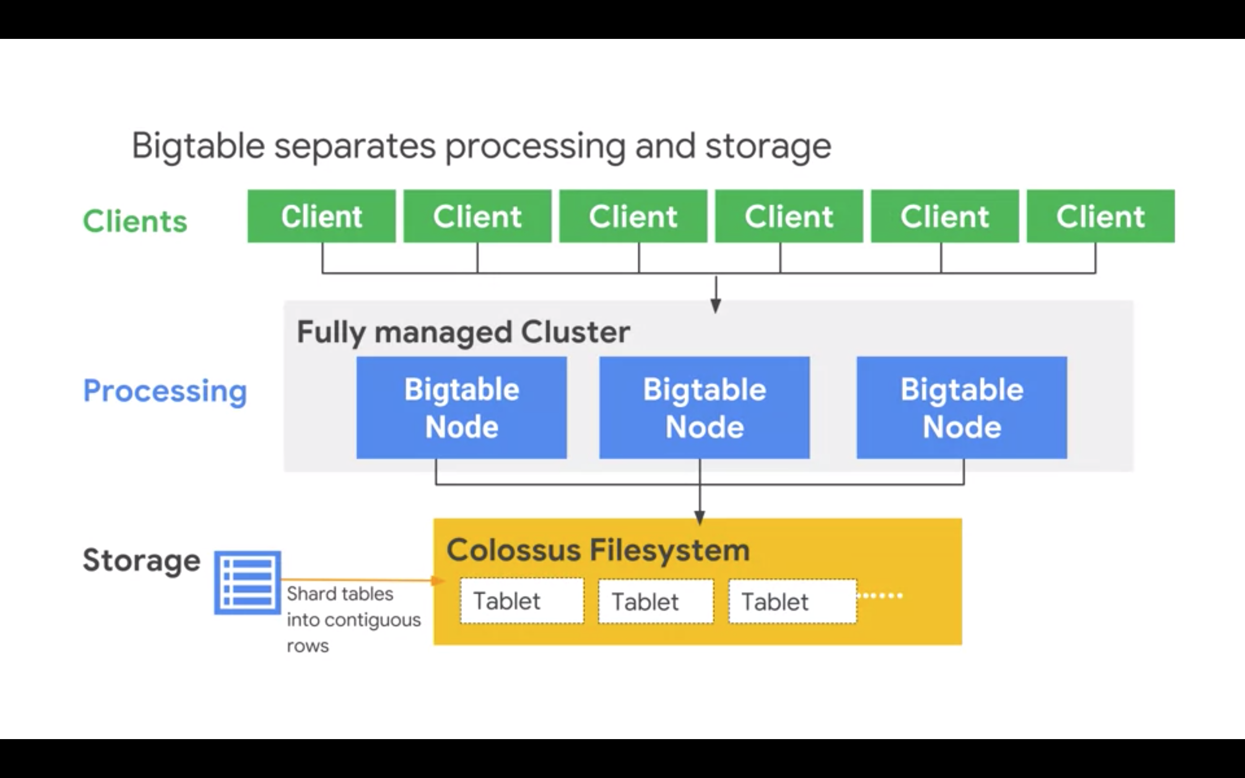
BigTable - big, fast, autoscaling noSQL, 100k QPS with 6ms latency for 10-cluster node. BT separates compute (running on nodes in clusters) and storage (in a form of tablets on Google Collosus on GCS). As such you can scale BT cluster on-the-fly after creation since data is separate.

Mutations to operate on BigTable. You can query BT from BQ.

Designing for BigTable

Only one index (row key). Column families grouping a set of columns belonging together or having similar type/cadence (things which never change or change often).

Two types of designs:

wide table, where each column exists for every row
narrow tables for sparse data

In BT rows are sorted lexicographically in ascending order of the row key.

Recommendations:

Queries that use the row key, a row prefix or a row range are the most efficient. Consider what is the most common query you need to support? This will help to define the row key. Store related entities in adjacent rows, so they are stored in similar tablets.
Add the reverse timestamp to the key, so you can get the “latest value” quickly
Distribute writes and reads across rows, so that workload across nodes is balanced. Bad examples: web domains (some will be more active), sequential like user IDs (new users are more active), static repeatedly updated identifiers (some will be more active).

Lab - Streaming into BigTable In this lab, you will perform the following tasks:

Launch Dataflow pipeline to read from Pub/Sub and write into Bigtable
Open an HBase shell to query the Bigtable database

Lab source

Create BT:

gcloud beta bigtable instances create sandiego --cluster=cpb210 --cluster-zone=us-central1-b --display-name=="San Diego Freeway data" --instance-type=DEVELOPMENT

Comminicating with BT with HBase </Lab>

Performance Considerations for BT

BT looks at the access patterns and reconsiders/optimizes itself, so it will take care of some level of hotspotting. Self-rebalance strategies:

distribute reads
distribute storage

Tips for improving performance:

design schema
don’t change schema too often to let BT optimize itself (couple of hours)
test it on at least 300Gb of data
SSD are faster than HDD (6ms vs 50ms at the time of training)
use from the same zone
control throughput with the number of nodes

Course 6 - Preparing for GCP Data Engineer Exam

Exam is testing practical skills rather than theoretical. Other similar certs are Cloud Engineer and Cloud Architect. Professional = Associate + design phase, business requirements and planning.

Top-down approach: key points, identify gaps, reach proficiency.

Case Study 1 - Flowlogistic

Start with Business Requirements. Look for generic terms to start shaping out the solution. Some immediate leads:

IoT Core for sensors
BigQuery for analytics with DataStudio for monitoring
Dataproc for existing Hadoop workflows

Move to Technical Requirements. When analyzing the existing environments focus on seven categories:

Location/Distribution: in this case it is in a single data center
Storage: various storage appliances like NAS
Databases: SQL, noSQL and Kafka in this case
Data processing: Hadoop/Spark in this case
Application servers: 60 VMs across 20 physical servers
Infrastructure: Jenkins, monitoring, security, billing
ML and predictive analytics: no existing environment

Coursera solution

Networking and connectivity VPC covering multiple regions. Cloud VPN for connection.
Applications Lift and shift to Compute Engine. Persistent disks? Persistent disks have lower IOPS than local disks.
Switch to GCP alternatives Kafka -> Pub/Sub Data collection -> IoT Core SQL -> Cloud SQL or Cloud Spanner Cassandra (wide-column noSQL) -> DataStore or BigTable
Hosted applications Depending on whether container-based can take to App Engine, K8S Engine or Compute Engine.
Static content Cloud storage with Content Delivery Network (CDN)
Misc items Batch server workloads Preemptible VMs with persistent disks (persistent have less IOPS) App Engine with Cron for repeated workloads Cloud Composer (Apache Airflow) for handling multiple processing pipelines Consider moving from Dataproc to Dataflow in Phase 2 Cloud Storage for images, Stackdriver Logging for Logs Backups: snapshots of persistent disks Datalake: cloud storage in place of HDFS, BigQuery eventually

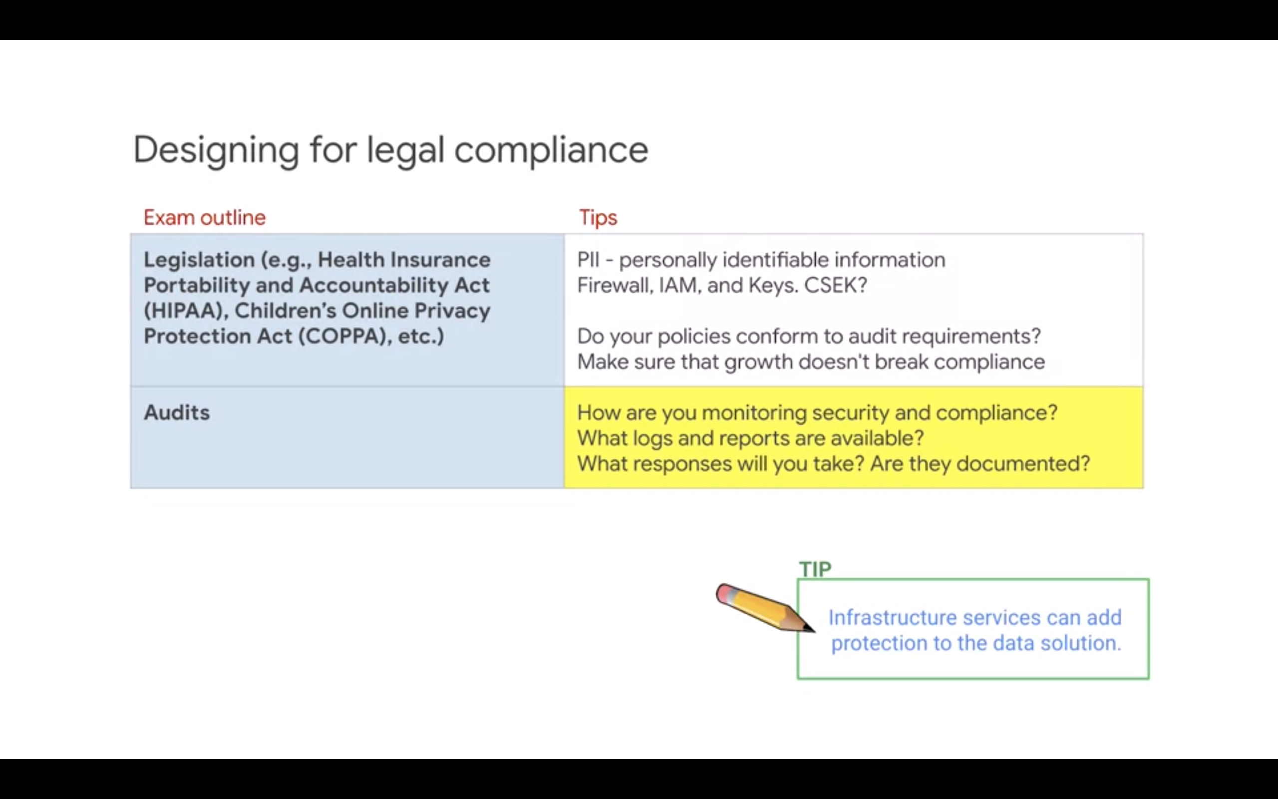
Case Study 2 - MJTelco

Search for keywords in business requirements:

minimal cost
security
reliability
isolated environments

Technical evaluation of existing environment:

Location/distribution: no environment
Proof of concept in the lab Nothing else is known, so let’s focus on the provided info and make reasonable assumptions on others.

Technical watchpoints:

network and log capabilities of their hardware, volume?
any ETL needed
type of data? structured, no-structured?

Coursera solution

Data ingest: Core IoT or secure file upload If applications: App Engine or K8S Engine, more scalable solution Datalake: BQ is structured and CloudStorage (multi-regional bucket) is unstructured Hadoop/Spark: multiple Dataproc clusters with access to same data for multiple environments Stackdriver for monitoring

Exam Tips

Need to know the basic information about each product that might be covered on the exam:

What it does, why it exists.
What is special about its design, for what purpose or purposes was it optimized?
When do you use it, and what are the limits or bounds when it is time to consider an alternative?
What are the key features of this product or technology?
Is there an Open Source alternative? If so, what are the key benefits of the cloud-based service over the Open Source software?

Touchstone concepts

Touchstone: “Unlike other vendor clouds, a subnet spans zones, enabling VMs with adjacent IPs to exist in separate zones, making design for availability easier to accomplish since the VMs can share tagged firewall rules.”

First part of exam covers design and building of data processing pipelines:

Data representation
Pipelines
Infrastructure

GCP ecosystem overview

Storage and databases: Storage

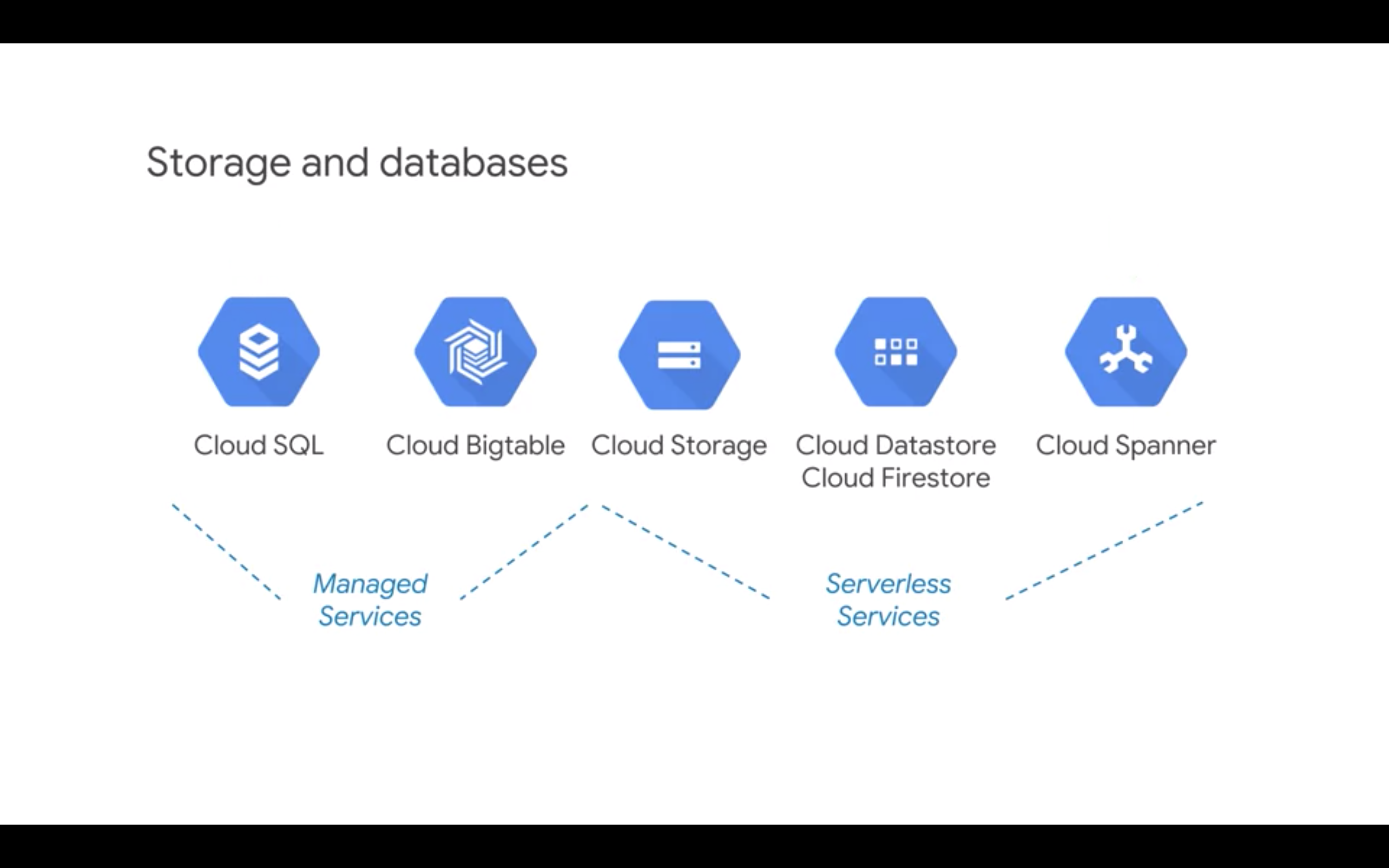
Cloud SQL and BigTable are managed services (i.e. you can see individual clusters or servers), so some IT
Cloud Storage, Datastore, Firestore and Spanner are serverless It is assumed that processing/compute is done outside of storage and databases.

Processing/computing: Compute

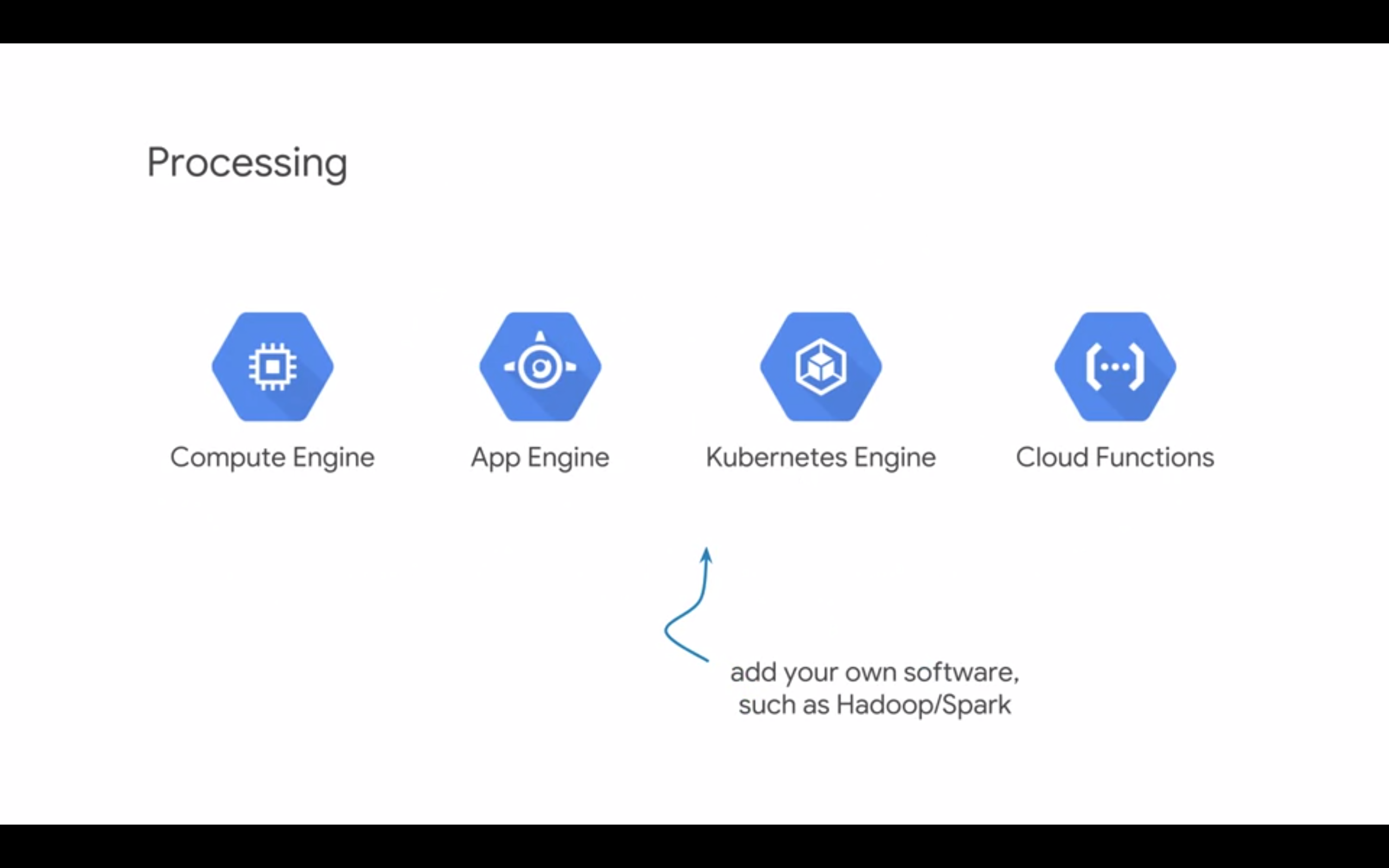
Compute Engine
App Engine
K8s Engine
Cloud Functions Each of these assumes that you provide your own business logic. All are managed, so there is an IT overhead.

Data Processing services:

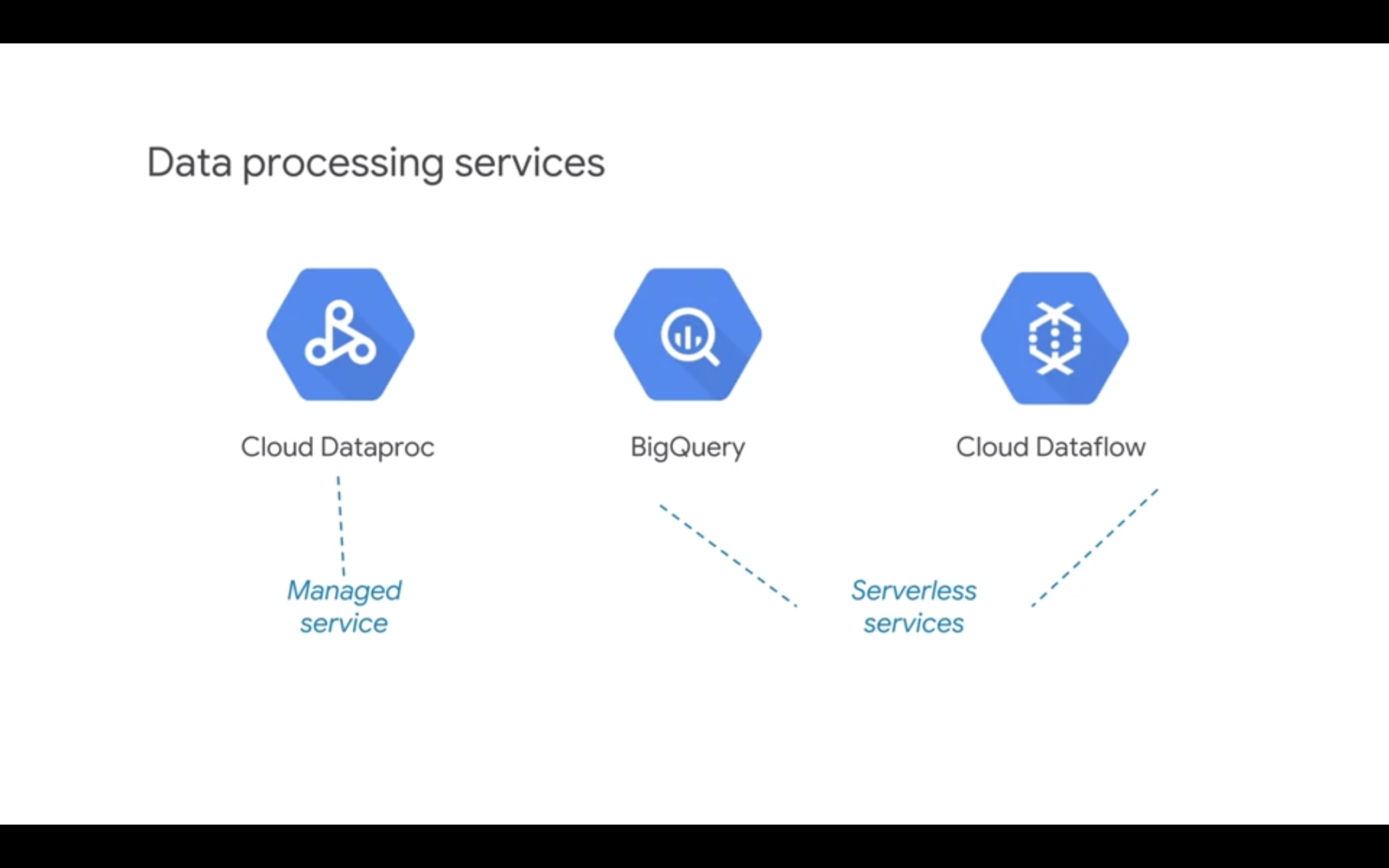
Dataproc (managed)
Dataflow (serverless)
BigQuery (serverless) Each of these overlap with each other. Data processing services combine storage and compute and automate the storage and compute aspects of data processing through abstractions. For example, in Cloud Dataproc, the data abstraction with Spark is a Resilient Distributed Dataset or RDD. The processing abstraction is a Directed Acyclic Graph, DAG. In BigQuery, the abstractions are table and query and in Dataflow, the abstractions are PCollection and pipeline.

Artificial Intelligence: 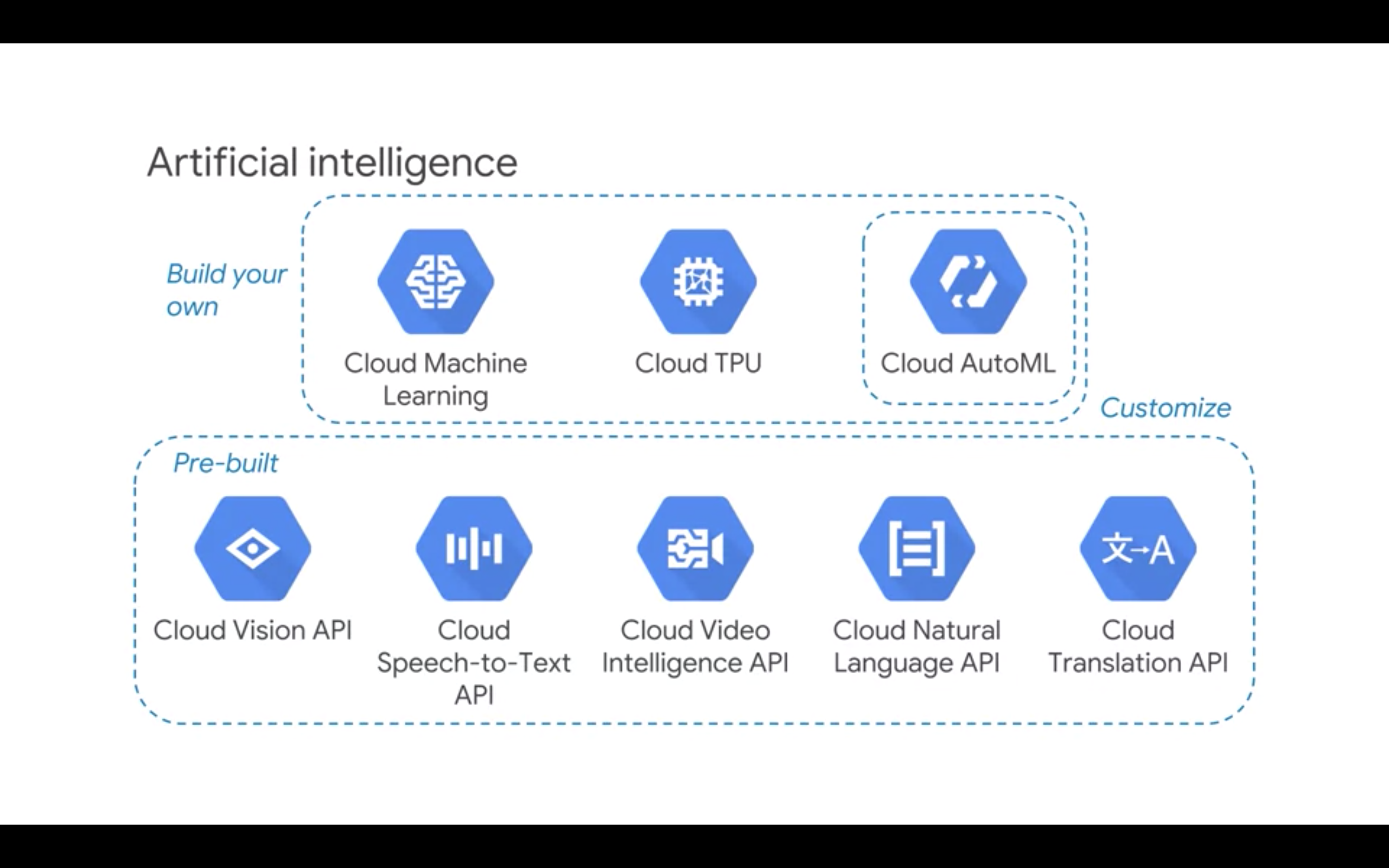Build your own: Cloud ML, Cloud TPU, Cloud AutoML Pre-built: Vision API, Speech-to-Text API, Video Intelligence API, NL API, Translation API

Preparing and Post-processing services: Pre- and post-processing

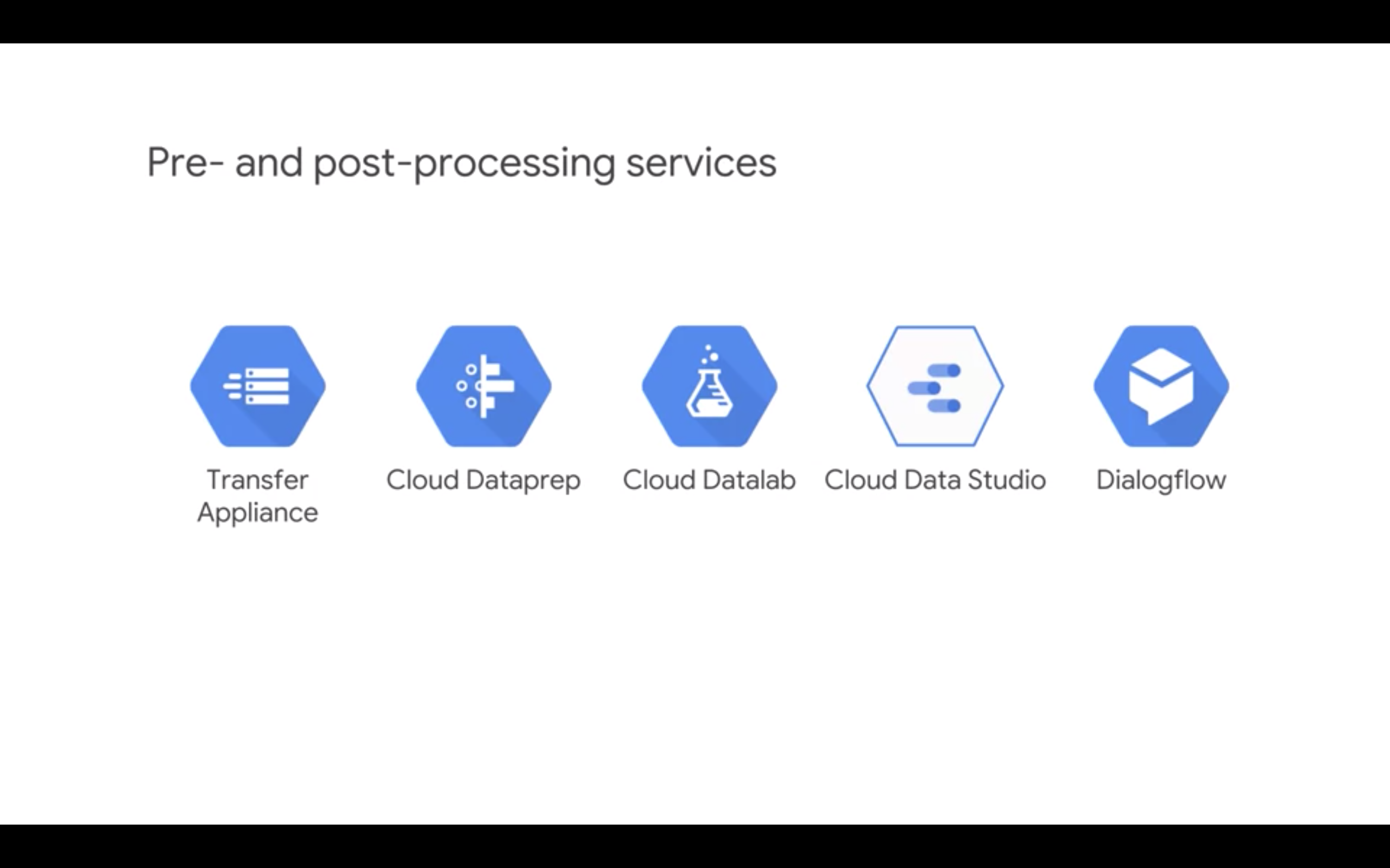
Data Transfer Appliance
Cloud Dataprep (by Trifecta)
Cloud Datalab (Jupyter)
Cloud DataStudio
Dialogflow

Infrastructure services: 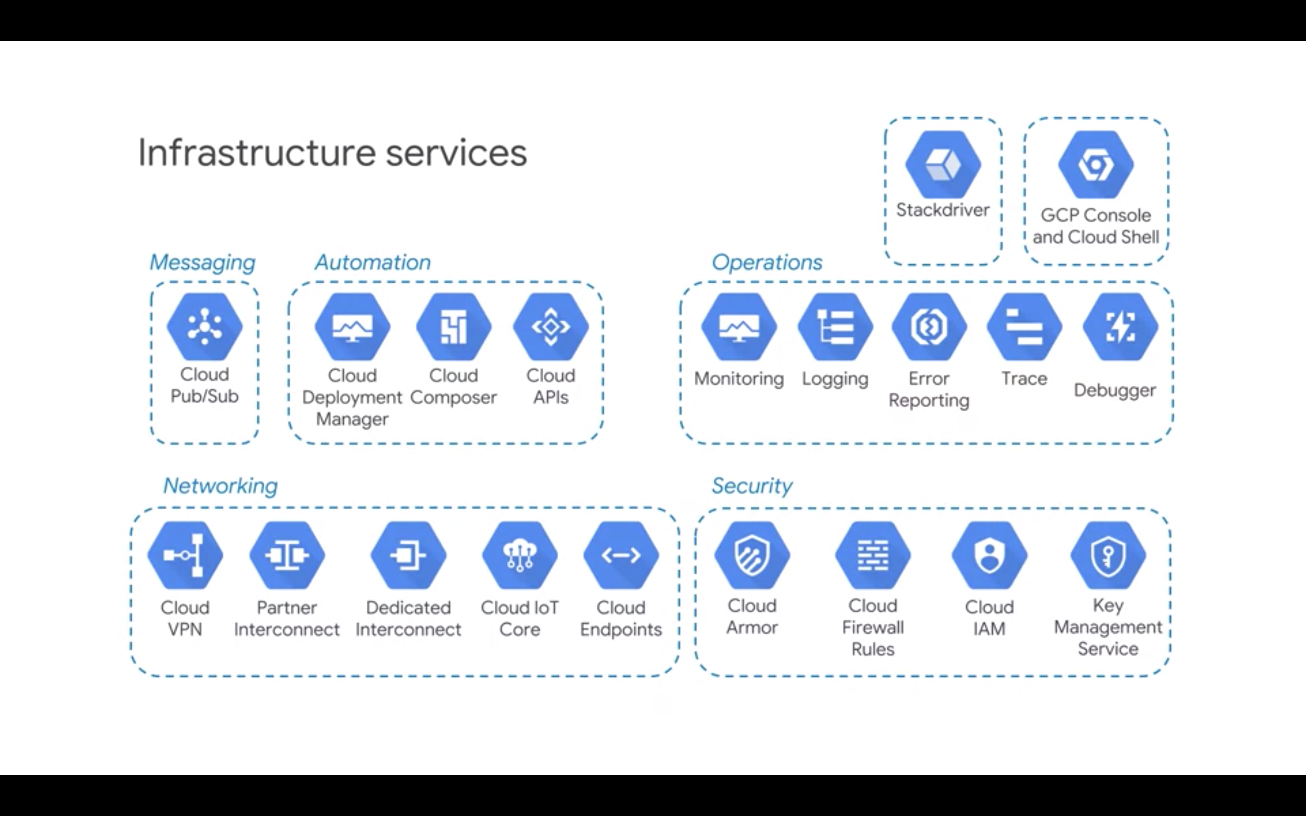Lots of services. No need to memorize exact IOPS and prices. However it is important to know the key differences, i.e. one service having higher throughput than other.

Flexible data representations

Exam Tip Know how data is stored in each system and what it is optimized for.

How you store data defines the best way to process it and vice-versa.

Cloud storage: data is object, stored in buckets (alternarive to OSS HDFS)
Datastore: data is property, contained in entity and is a kind category
CloudSQL: values in rows and columns in table in database
Cloud Spanner: same as above

AVRO Avro is a remote procedure call and data serialization framework developed within Apache’s Hadoop project. It uses JSON for defining data types and protocols and serializes data in a compact binary format.

BigQuery Data in tables in datasets (access control), which are inside project (same billing, etc). BQ is columnar, which is cheaper than row processing. Queries use only few columns usually. Also every column is same type, so BQ can compress it very effectively.

Spark Data is stored as an entity, but behind the scenes it is in Resilient Distributed Dataset (RDD), which is managed by Spark itself.

Dataflow Data is represented as PCollection. Each step is a Transform. Many Transforms form a Pipeline. Pipeline is executed by the Runner (local or cloud for production). Each Transform uses a PCollection and returns a PCollection, so PCollection is the unit of data. Unlike Dataproc Dataflow is serverless.

PCollection is immutable and this is the source of the speed in Dataflow processing. Dataflow uses same code and pipelines for Batch and Streaming data. Averaging for streaming is done by selecting Window length, for instance.

Tensorflow Data in TF is represented as Tensors. Tensor 0 is single value, Tensor 1 is vector and so on.

Data pipelines

Dataproc consideration

Dataproc

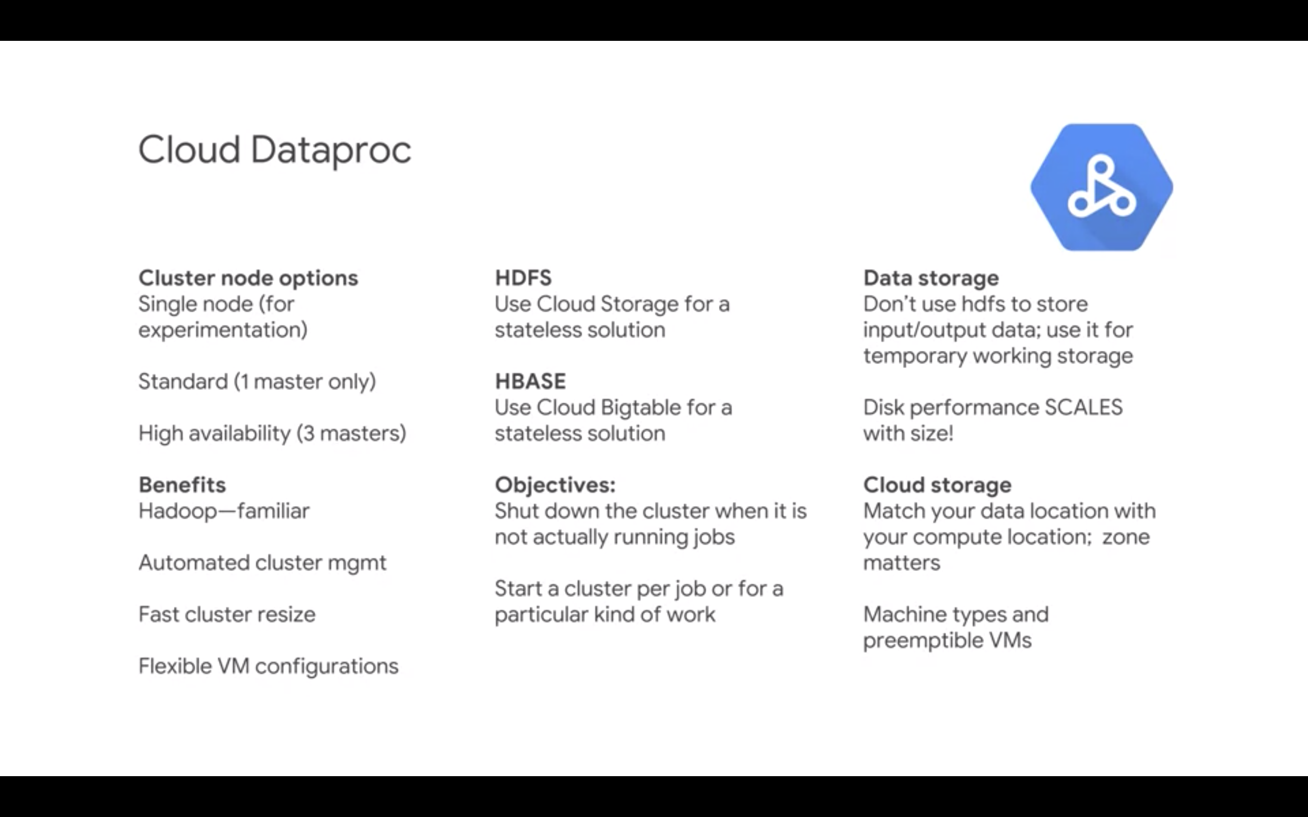
It is recommended to use stateless Dataproc cluster by storing data externally (BT/HBase, Cloud Storage/HDFS), so you can shut it down when not in use.

Exam tip Spark does some of it processing in-memory, so for certain tasks it is extremely fast.

Dataproc Spark RDD use lazy evaluation. It builds DAGs, but waits till the requests are made to allocate resources. Dataproc can augment BQ by reading from it, processing and loading back. Dataproc has multiple connections to read/write from many GCP services.

Use initialization actions during cluster startup to prepare clusters.

Exam tip If data is in BQ and business logic is better expressed as a code, rather than SQL it may be better to run Spark on top of BQ.

Dataflow considerations

You can get data from many sources and write to many sinks, but pipeline code remains the same (Java, python) and also is valid both for streaming and batch. Dataflow transforms can be done in parallel.

Some of the most common Dataflow operations: ParDo, Map, FlatMap, apply(ParDo), GroupBy, GroupByKey, Combine. Know what are the most expensive (GroupByKey).

Template workflows to separate developers from users.

Exam tip User roles to limit access to only Dataflow resources, not just the project.

Infrastructure

BQ has two parts: frontend for analysis, backend for storage.

Exam tip Know the BQ access control granularity - projects/datasets.

Separation of compute and storage allows for serverless operations, i.e. BQ can run analytics on multiple data sources. This is completely opposite to Hadoop/HDFS and became possible because of petabyte network speeds within GCP.

Cloud Dataproc follows the same logic of splitting compute and storage, so now it is possible to shut down cluster when not in use. Know the analogy of BT=HBase, GCS=HDFS.

Cloud Dataflow is an ETL solution for BQ.

Various Data Ingestion patterns: (https://omdv.github.io/assets/GCP_exam-data-ingest.png) BQ ingest (https://omdv.github.io/assets/GCP_exam-BQ-ingest.png)

Exam tip Use gsutil when transfering from on-premise, use Storage Transfer Service when moving from another cloud provider.

Exam tip Cloud Pub/Sub will hold messages up to 7 days.

Typical patterns:

Cloud Pub/Sub for ingestion
Cloud Dataflow for processing
BQ for analysis

Pipeline example (https://omdv.github.io/assets/GCP_exam-infra-example.png)

Some other tips for this section:

Tips 01 (https://omdv.github.io/assets/GCP_exam-tips-01.png) Tips 02 (https://omdv.github.io/assets/GCP_exam-tips-02.png) Tips 03 (https://omdv.github.io/assets/GCP_exam-tips-03.png)

Building and Maintaining Solutions

CAP Theorem, ACID vs BASE:

CAP is Consistency, Availability, and Partition tolerance. You can pick 2 of those but you can’t do all 3.
ACID focuses on Consistency and availability.
BASE focuses on Partition tolerance and availability and throws consistency out the window.

Cloud Storage: be familiar with all access control methods, like IAM, signed URL, etc. Know about storage classes, lifecycle management.

Cloud SQL vs Cloud Spanner. Spanner is globally consistent and can support much bigger size. Distributing mySQL is hard, so Spanner is the solution.

Cloud Datastore was previously available only for AppEngine, but now can be used outside.

Storage 01 (https://omdv.github.io/assets/GCP_exam-storage-options.png) Storage 02 (https://omdv.github.io/assets/GCP_exam-choosing-storage.png)

Dataflow: know triggers, watermark, different windowing types, side inputs, etc.

Storage 03 (https://omdv.github.io/assets/GCP_exam-data-processing-solutions.png)

Exam tip To move data from one location in BQ to another - use the GCS bucket and change the region of the bucket before creating a new dataset.

Exam tip When considering pipelines look at business requirements for consumption frequency, look for in/out sides. How frequently and how significantly the demand for resources will change (i.e. serverless vs server).

Analysis and Modeling

Cloud Datalab to explore and develop.

Cloud ML engine:

Train data
Create trainer and make it available to Cloud ML
Conf and start a CloudML job

Tensorflow: be familar with levels and some key functions. Lazy mode vs eager mode.

Exam tip Know supervised vs unsupervised, regression vs classification, loss functions (RMSE vs MSE), etc. Goal is “practical, not perfect”.

Exam tip Confusion matrix to measure the performance of classification models. Be able to distinguish toy ML solutions from production solutions.

Normalization - the trade off between relationalism and flat structure. Flat structure in general provides better scalability, i.e. the example of adding a new column to the schema. Normalized is more efficient (storage-wise), denormalized (more repeated fields) is more performant.

BQ can use nested schemas.

Grouping a highly-cardinal data is a bad idea.

BigTable performance

Bigtable

Row key design (refer to the related course): use reverse timestamp with some additional category, so that queries are distributed.

Performance increase (QPS) is linear with the number of nodes. Adding new nodes may take few hours to propagate to have an impact on performance.

BigQuery pricing

Loading is free. Avoid “select ALL”, as it will drive the cost significantly. Use the costing calculator.

Reliability and Non-Functionals

Scaling may improve the reliability. Quality control - monitor in Stackdriver or DataStudio.

Exam tip Some quality control features can be built into the technical solutions, e.g. using TFBoard to monitor the quality of training on validation set.

Review DS terminology - filters, dimensions, views, metrics, etc.

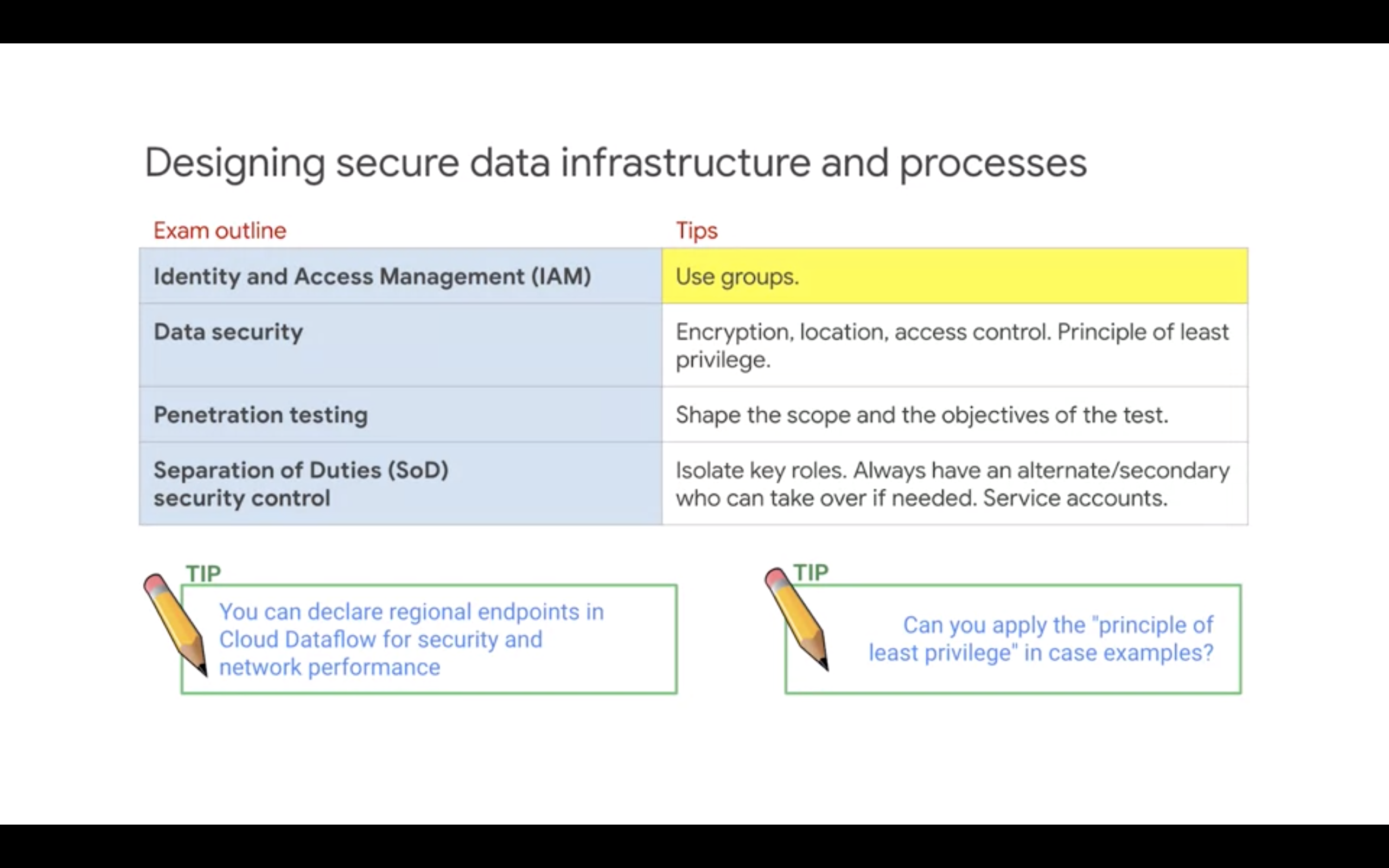
Security

Be aware of the granularity of control for each service.

Various encryption methods:

default (managed encryption)
customer-managed encryption keys (cmek)
customer-supplied EKs (csek)
client-side encryption

Know key concepts: Cloud Armor, Cloud Load Balancing, Cloud firewall rules, service accounts, separation into front-end and back-end, isolation of resources using separate service accounts between services.

Exam tip Determine the service at question, determine the level of security requirements.

Exam tip BQ authorization is at dataset level. To give access only to queries and not the underlying dataset - export results of the query to a diff dataset and give access to it instead.

Security-01 Security-02

Challenge Lab - 1

Create a query that produces the average trip time for trips originating from the airport in Frankfurt, Germany (FRA) and destined for the airport in Kuala Lumpur, Malaysia (KUL), and group the results by airline. The resulting average times should be similar.

SELECT
  airline, AVG(minutes)
FROM 
  `qwiklabs-gcp-02-e9b65681da2f.JasmineJasper.triplog`
WHERE
  origin='FRA' AND destination='KUL'
GROUP BY
  airline

Create a query that produces the average trip time for trips originating from London Heathrow Airport, United Kingdom (LHR) and destined for the airport in Kuala Lumpur, Malaysia (KUL), and group the results by airline, and order them from lowest to highest. The resulting average times should reveal whether the airline, PlanePeople Air, kept its promise to use faster airplanes from Heathrow Airport.

SELECT
  airline, AVG(minutes)
FROM
  `qwiklabs-gcp-02-e9b65681da2f.JasmineJasper.triplog`
WHERE 
  origin='LHR' AND destination='KUL'
GROUP BY
  airline
ORDER BY
  AVG(minutes) ASC

Challenge Lab - 2

Create a cluster with access to a Cloud Storage staging bucket. Run PySpark jobs with input arguments. Troubleshoot and resolve a cluster capacity job error. Upgrade the master node configuration on an existing cluster. Resolve a cluster capacity performance issue. Upgrade the number of worker nodes on an existing cluster.

Resources for Further Reading/Preparation

Know high-level description of each of the services below.

Storage and Database services: 1.1 Disks 1.2 Cloud Storage 1.3 Cloud Memorystore 1.4 Cloud SQL 1.5 Cloud Datastore 1.6 Cloud Firestore 1.7 Firebase Realtime Database 1.8 Bigtable 1.9 Spanner
Data Analytics 2.1 BQ 2.2 Dataflow 2.3 Dataproc 2.4 Datalab 2.5 Dataprep 2.6 Pub/sub 2.7 Data Studio 2.8 Composer
ML 3.1 Cloud ML Engine 3.2 TPU 3.3 AutoML 3.4 Natural Language 3.5 Speech-to-Text 3.6 Translation 3.7 Text-to-speech 3.8 Dialogflow Enterprise 3.9 Cloud Vision 3.10 Cloud Video Intelligence
Infrastructure 4.1 StackDriver 4.2 Transparent Service Level Indicators 4.3 Cloud Deployment Manager 4.4 Cloud Console

Also:

DE Practice Exam on GCP.
Qwiklabs Data Engineer Quest

Review of tips: TIP 1: Create your own custom preparation plan using the resources in this course. TIP 2: Use the Exam Guide outline to help identify what to study. TIP 3: Product and technology knowledge. TIP 4: This course has touchstone concepts for self-evaluation, not technical training. Seek training if needed. TIP 5: Problem solving is the key skill. TIP 6: Practice evaluating your confidence in your answers. TIP 7: Practice case evaluation and creating proposed solutions. Tip 8: Use what you know and what you don’t know to identify correct and incorrect answers. Tip 9: Review or rehearse labs to refresh your experience Tip 10: Prepare!

Course 1 - Google Cloud Platform Big Data and Machine Learning Fundamentals

Course 1.1 - Introduction to GCP

Compute

Storage

Networking

Security

Evolution of GCP

Links

Course 1.2 - Recommending System using Spark and Cloud SQL

Links

Course 1.3 - Predict visitor purchases with BigQuery ML

BigQuery ML

Course 1.4 - Create Streaming Data Pipelines with Cloud Pub/sub and Cloud Dataflow

Links

Course 1.5 - Classify Images with Pre-Built Models using Vision API and Cloud AutoML

Links

Course 2 - Leveraging Unstructured Data

Course 2.1 - Introduction to Dataproc

Choosing the right size of your VMs

Course 2.2 - Running Dataproc jobs

Networking

Submitting Spark jobs

Leveraging GCP when working with Dataproc - BigQuery and Cluster Optimization

Links

Course 3 - Serverless Data Analysis

Course 3.1 - BigQuery

Loading and Exporting Data to BigQuery

Advanced Capabilities in BigQuery

Performance and Pricing

Course 3.2 - Dataflow

MapReduce in Dataflow

Side Inputs in Dataflow

Links

Course 4 - Serverless Machine Learning with TensorFlow

Course 4.1 - Intro in Machine Learning

Links

Course 4.2 - Intro to TensorFlow

Course 4.3 - CloudML Engine

Packaging TF trainer

Links

Course 4.4 - Feature Engineering

Links

Course 5 - Building streaming systems on GCP

Course 5.1 - Streaming scenarios

Course 5.2 - Ingesting variable volumes

Course 5.3 - Dataflow streaming

Course 5.4 - Streaming analytics and dashboards

Course 5.5 - Handling throughput and latency requirements

Designing for BigTable

Performance Considerations for BT

Links

Course 6 - Preparing for GCP Data Engineer Exam

Case Study 1 - Flowlogistic

Case Study 2 - MJTelco

Exam Tips

GCP ecosystem overview

Flexible data representations

Data pipelines

Infrastructure

Building and Maintaining Solutions

Analysis and Modeling

BigTable performance

BigQuery pricing

Reliability and Non-Functionals

Security

Challenge Lab - 1

Challenge Lab - 2

Resources for Further Reading/Preparation

Links