Udacity Artificial Intelligence Nanodegree
Term 1 - Search and Planning
Lesson 2: Refresher and setting up
Math refresher (optional):
Lesson 4: Intro to AI
AI is a moving target, e.g. chess, path finding, chatting agents, so on.
Heuristic - additional logic, constraint which prompts brute-force to act more effficiently. Astar is an improvement over Dijkstra due to heuristic.
When choosing the best representation for the game model choose the one moving the problem to action-solution space in a way. E.g. for tic-tac-toe use every position as a node and edges between them if there is a legal move. Pruning the search tree with the help of heuristics
Mini-max search and adversarial search - maximizing your chances during your turn and opponent minimizing chances during their turn. Definitions of agent, environment, states and goal state. Agent has perception to interact with environment, use cognition to take action to change environment. Intelligent agent is the one that takes actions to maximize it’s utility given a desired goal, i.e. rational behavior, however agent cannot behave optimally always, so we define “bounded optimality” to quantify the intelligence.
Links:
Lesson 5: Applying AI to Sudoku
Encoding the problem, coordinates, peers based on the rules we want to implement later Techniques:
- Elimination
- Only choice (i.e. in 3x3 square)
Links:
Lesson 8: Playing Isolation game
- Book of opening moves. How to choose best opening automatically - minmax algorithm.
- Min and max levels - our bot is trying to maximize his chances and opponent always plays perfectly to minimize it.
- Branching factor and depth of the search tree to estimate the time required to solve the game
- Typically b^d is too large to completely explore the whole tree
- Depth-limited search to estimate the max-depth for a given average branching factor to have acceptable “wait time”
- Start from the bottom of the tree. For each max node pick the maximum value along the child nodes, and vice-versa.
- Quiescent search - sensitivity analysis as to how results change based on how many level limitations we have. Choose the one after which results are stable.
Lesson 9: Advanced Game Playing
- Iterative deepening - include next level consideration only if time allows
- Depth of possible search with ID may vary with branching factors and be different in different phases of the game
- Horizon effect
- Explore other evaluation functions and choose best for the game
- Alpha-Beta pruning - ignore subtrees which do not change results at higher tree level.
- Tips for 5x5 Isolation agent - symmetry, book of opening moves, reflection, separation, order nodes correspondingly to optimize pruning
- Multi-player isolation - no minimax, propagate values based on each players selection at every level
- For probabilistic games just add a probability for each branch and do minimax with probability accounted for
Lesson 11: Search
- Definition of a problem (states, actions, goals, costs, etc)
- Frontier, explored region and unexplored region
- Tree search methods are similar, the difference is in how you choose the action
- Breadth-first search - shortest path always, first found may suffice and be a solution (one of)
- Uniform cost (or cheapest first) search - continues to search until the path is removed from frontier, guaranteed
- Depth-first search - expand the longest path first, not guaranteed to find the optimal path
- All the above algos are non-efficient time-wise as they explore in all directions, need additional knowledge
- The best knowledge for search is distance to the goal
- Greedy best-first search uses the distance, effective but cannot handle barriers
- A* - minimum of g+h (path cost + distance of the final state of the path to the distance to the goal), could also be called best estimated total path cost first
- For Search to work domain should have some characteristics: fully observable, known (know available actions), discrete (a limited set of actions to choose from), deterministic (know the result of taking an action), static (only our actions change the world)
- To implement we define node with state, action, cost and parent, frontier is defined as set, should be able to remove members, add new and do a membership test, priority queue.
Lesson 12: Simulated Annealing
- Techniques to solve very complex problems by trying simple heuristics first
- Example of travelling salesman of n-queens problems - initiate randomly, move pieces with largest number of conflicts and iterate
- The issue is the local maxima/minima, solution is to do a random restart
- Random restart with many attempts. Use Taboo search to avoid areas which were explored
- Step-size selection - typical for optimization problems
- Simulated annealing - “heating” and “cooling” the system to achieve the “minimum energy level” or global minima/maxima. Heating in this context means increasing randomness and cooling vice versa.
- Local beam search - variation of random restart but with N particles, which further exchange information between them by being compared. We choose only the best.
- Generic algorithms - crossovers, mutation, etc
Lesson 13: Constraint Satisfaction
- Constraint optimization techniques - backtracking optimization and forward checking.
- Some heuristics may be applied to backtracking, such as least constraining value, minimum remaining values
- Structured CSPs - tricks to divide problem into smaller pieces or acyclic graphs to reduce complexity
Lesson 14: Login and Reasoning
- Peter Norvig’s vision of future directions for planning algorithms: learning from examples, transfer learning, interactive planning (human + machine), explaining things in terms human can understand
- Propositional logic to define models between events/variables. Truth tables.
- Limitations of P.L. - can handle only binary values, can’t handle uncertainty, can’t cover physical world objects, no shortcuts to cover many things happening at the same time
- First order logic extent P.L. as it introduces relations, objects and functions which can describe the world, while P.L. had only facts
- FOL models contain constants, where multiple constants can refer to the same object and functions, which map objects to objects
Lesson 15: Planning
- Planning requires some interaction with the environment during execution phase
- In stochastic worlds it is helpful to operate in the space of belief states
- Conformant plans require no information about the world
- Partially observable world
- In stochastic environments actions tend to increase the uncertainty, while observations tend to bring it back down
- Classical planning representation: state space, world state, belief state, action schema (part 12)
- Progression state search
- Our classical planning representation allows us to use regression search
- Regression vs progression - depends on the goal
- Plan space search - used to be popular in 1990s.
- Forward search is more popular now, because it allows to come up with better heuristics
- The classical planning representation allows to do automatic heuristics search by relaxing some of conditions automatically and search through it
- Situation Calculus - can’t apply Classical Planning to all cargo. S.C. allows it with First Order Logic
Lesson 16: Probabilities & Bayes Networks
Bayes networks are the building blocks of more advanced AI techniques, like particle filters, Kalman, etc. Conditional probabilities refresher.
Lesson 17: Bayes Nets
- Bayes nets statement:
- We know the prior about A - P(A), but A is not observable
-
B is observable and we know P(B A) and P(B notA) -
We need to do the diagnostic reasoning, i.e. P(A B) and P(A notB) - Two test cancer quiz:
-
P(C)=0.01, P(+ C)=0.9, P(+,!C)=0.8, P(C ++)? - Using tabular approach is the easiest
-
P(++ C) = P(+ C) * P(+ C) assuming conditional independence - Other techniques - conditional independence, total probability conditioned on 1
- Explaining away - if there is an effect explained by multiple causes and one cause is already observed then it is less likely that other causes had an effect
-
Complex conditional probabilities like P (A B,C) can be expanded using simple Bayes rule, i.e. P(A B) = P(B A)P(A)/P(B) where all variables are given C, i.e. p(A B,C) = p(B A,C)p(A C)/p(B C) - Bayes nets use the graph representation which allows to represent complex networks with small number of joint probability distributions
- D-separation for independence, explain away may bring dependence into a pair of previously independent variables
Lesson 18: Inference in Bayes Nets (Exact inference)
- Evidence, query and hidden variables
-
We are looking for probability of one or more query variables given some values for one or more evidence variables - P(Q1, Q2 E1=e1, E2=e2) - Enumeration technique, but can be slow for large bayes nets
- Speeding up techniques: Pulling out, maximizing independence
- Bayes nets are the most compact and easiest to work if they are written in causal direction
- Variable elimination technique - step by step factor multiplication
Approximate Inference
Use sampling to get joint probability distributions. This also let us build the conditional probability tables. Gibbs sampling using MCMC
Lesson 19: Hidden Markov Models
- Time series pattern recognition
- A lot of human activities fall in domain of pattern recognition through time series
- How to match two signals - use delta frequency for freq matching and dynamic time warping for matching across time
- HMM training - break your sequence into a number of states, calculate prob distribution, calculate transition probabilities, update boundaries and so forth until convergence
- Baum Welch - variation of the expectation maximization process
- Any distribution may be represented by a mixture og Gaussians
- Choosing HMM topology
- Different specific tricks: Context grammar and statistical grammar combined reduce the error rate by 8
- HMMs are generally bad for generating data, while good at classifying it - the problem is that the output has no continuity.
Links:
Term 2 - Deep Learning
Generic Notes
Taken during watching the lectures, also I knew most of it from before, so it is somewhat chaotic.
Week 1: Deep NN
- Usual NN explanations - AND, OR, NAND, XOR, etc
- Using graphical representation to explain the separation of classes
- Moving line towards misclassified points with learning rate
- Error functions, gradient descent, error function needs to be continuous for GD
- Sigmoid is needed vs step function to give a continuous change, good explanation of activation functions overall
- Softmax for multiclass problems - normalized exponents of linear outputs
- One-hot encoding
- Maximum likelihood (log-likelihood is required to get rid of products of probabilities)
- Cross-entropy is the negative sum of log of probabilities. Good model - low cross-entropy. Misclassified points have higher negative log of probability, because log of probability of 1 is zero. Cross-entropy is the sum of all outcome probabilities times the outcome for all samples. Essentially we are adding probabilities only of the events that have occured by multiplying log of probability by the label for the event.
- Logistic regression - explanation is based on error function described earlier, which is a mean of log of probabilities times label
- Gradient descent calculations - analytical derivations. For logistic regression the gradient turns out to be just the scalar times coordinates of the point, where scalar is just the difference between the label and the prediction. Updating weights and bias becomes as simple as just multiplying learning rate (normalized by number of points) by coordinates. GD algo is similar to previously discussed Perceptron algo.
- Perceptron just draws a line or hyperplane given weights for each input and bias and determines if given point is positive or negative (activation function -> sigmoid vs step function)
- Neural networks (or MLP) - combining first level models to get more complex models, using weights for previous models to achieve the right combination, applying activation functions (sigmoid) to get continuous probability and also cut-off probability at one.
- NN architecture - nodes equal to problem dimension, output equal to a number of classes needed to be classified.
- Feedforward - forward calculation to get the error function for the whole network
- Backprop - feedforward with gradient descent. Calculating derivatives at each layer, use chain rule for derivatives.
- Bias vs variance - it is better to stay on overcomplicated side and implement some techniques to prevent overfittting
- Early stopping - stop when test error starts to increase
- Regularization - we don’t want too certain models, because their activation function has too steep curve in the vicinity of zero and as such are difficult to be handled by gradient descent. Large coefficients cause the overfitting. Regularization punishes big coefficients. L1 or L2 regularization. L1 regularization is better for feature selection, L2 is better for training models.
- Dropout - randomly turning off some nodes during the training to let other nodes train and train the whole network more uniformly.
- Vanishing gradient with sigmoid function - either tanh or relu.
- Random restarts to solve the local minimum problem.
- Momentum to skip small humps to not get stuck in local minima - work really well in practice.
Week 2: CNNs
- Google’s wavenet - reading text
- MNIST MLP notebook best practices:
- one-hot encode and flatten
- relu, rmsprop
- use ModelCheckpoint callback and validation split when training
- CNNs are similar to MLPs in activation functions, however use different hidden layers to address the following two issues of MLPs:
- MLPs use only fully connected layers, so the number of parameters is too high
- We throw away the 2D info contained in the image when we flatten it, i.e. the underlying spatial info of the image is lost
- CNNs use the layers, which are sparsely connected and informed about 2D structure
- Locally connected layers vs densely connected layers
- Convolutional layers:
- the node value is a sum of weights times the value of pixel/input, apply ReLu
- weights can be represented in a grid, with the size matching the size of the convolutional windows, then this grid is called a filter
- filter resembles the pattern it is designed to detect, so it is useful to visualize the filter to understand what type of pattern it will detect
- convolutional layer may have multiple collections of filters to look after different patterns
- with this said in CNNs we do not pre-specify filters, CNN will learn the best filters based on the images it needs to detect
- Collection of filters is called either a feature map or activation map
- For color images the filter becomes the stack of three 2d matrices, one for each color in RGB, the multiplication of input by filter weights is done for each color correspondingly
- Hyperparameters of convolutional layers:
- size of filters
- number of filters
- stride of filters - step by which we move filter across the image. Stride of one will create roughly the same size layer as the image, stride of two will create approximately the half, approximately because of the edge. You could either ignore the size mismatch and you may loose some nodes, otherwise you can pad image with zeros.
- Number of parameters in conv layer is: n_filters * size_filter^2 * depth_input + n_filters (for bias)
- Depth of the output of layer is equal to n_filters
- Shape depends on padding and stride
- Pooling layers are the second type of layer for CNN, required to reduce dimensionality or complexity of conv layer output. There are many different types. Max pooling will use the window of some size and select max value in the specific window. Global averaging PL will just average each layer/filter of conv.layer and return just a vector. All pooling layers will still have the number of outputs (be it matrix or single value) equal to the initial number of layers/filters.
- Pooling usually has either max or average, 1D, 2D, 3D and global vs window-based
Week 4: End of CNN and TF intro
- CNNs require images of the same size. It is typical to transform all images to square with dims of power of two
- CNN progression may be seen as a start with 2D image with depth (1 for grayscale, 3 for RGB). CNNs then progressively increase the depths. Convolutional layers increase the depth due to the addition of filters and may also decrease spatial dimensions, pooling layers keep the depth the same and decrease dimensions significantly depending on the type of pooling.
- Some typical values:
- filters/kernels size are 2x2 to 5x5
- stride is usually 1 (default)
- padding is better “same” (not default)
- combined above results in the layer of the same size, but increased depth
- conv layers connected in series typically have increasing number of filters
- The intuition is that as you combine conv layers of increasing depth with max pooling you convert spatial information into a depth, where each layer in a final pooling layer may be seen as answering questions about the image, like whether there are wheels, or legs or eyes. We don’t prespecify these questions as we don’t specify the type of filters, instead the model creates the “right questions” itself.
- The final pooling layer may be flattened, because all spatial info is already preprocessed and lost at this point. Then the dense layer with relu and final layer with softmax may be used.
- Image augmentation - generate synthethic test data by rotating, flipping and translating your training images. Keras has corresponding functions, the fit method is slighly different as well.
- ImageNet competitions milestones:
- 2012: AlexNet introduced dropouts and ReLus
- 2014: VGG pionered the use of smaller filters. They used 16 or 19 layers total with 3x3 filters grouped in three blocks of conv layers separated by pooling layers
- 2015: ResNet has 152 layers. Usually this is a problem because of vanishing gradient problem. ResNet resolved it by implementing a shortcuts between layers to let the gradient backpropagate.
- Most of the winning architectures and trained nets are accessible through Keras
- Techniques to understand how CNN works:
- showing the output of each filter real-time
- constructing images which maximize the activation of a layer - famous illustrations. Then it may become apparent what a layer is trying to distinguish, say a building or eyes or legs, etc.
- Deeper layers may provide a more refined representation, while first layers may be looking at just simple patterns
- Transfer learning is a technique to use pre-trained CNNs for your specific classification tasks. CNNs are trained to detect patterns, so if you remove only the last (few) layers which are responsible for detection of specific objects and add dense layer to train to your new dataset it is possible to re-train network. There are different strategies on how to do it, depending on the size of your dataset and how much the new task differs from the one used to train the original network.
Links:
- Stanford course on CNN
- Activation functions
- Understanding CNNs
- Deep Vis Toolbox
- Stanford DL wiki
- More on CNN filters intuition
- Keras callbacks
- Karpathy’s on deep RL
- Deep Learning as a black magic
Lesson 8: Tensorflow
Hello World
Tensorflow Hello World script:
import tensorflow as tf

# Create TensorFlow object called tensor
hello_constant = tf.constant('Hello World!')

with tf.Session() as sess:
    # Run the tf.constant operation in the session
    output = sess.run(hello_constant)
    print(output)
Data as Tensors
In TF data represented as tensors, so tf.constant is 0-dimensional string tensor. Other examples:
# A is a 0-dimensional int32 tensor
A = tf.constant(1234)
# B is a 1-dimensional int32 tensor
B = tf.constant([123,456,789])
# C is a 2-dimensional int32 tensor
C = tf.constant([ [123,456,789], [222,333,444] ])
TF session is an environment to run a computational graph, in the example above we call it to evaluate the hello_constant.
Variables, Placeholders, Constants
tf.placeholder() returns a tensor that gets its value from data passed to the tf.session.run() function, allowing you to set the input right before the session runs. To pass data use feed_dict in session.run().
x = tf.placeholder(tf.string)
y = tf.placeholder(tf.int32)
z = tf.placeholder(tf.float32)

with tf.Session() as sess:
    output = sess.run(x, feed_dict={x: 'Test String', y: 123, z: 45.67})
TF math requires specific operators, like in the example below:
x = tf.constant(10)
y = tf.constant(2)
z = tf.subtract(tf.divide(x,y),1)

# TODO: Print z from a session
with tf.Session() as sess:
    output = sess.run(z)
    print(output)
tf.constant() and tf.placeholder() cannot be modified, so we need a Tensor which can be modified. tf.Variable class allows it. tf.Variable needs to be initialized before running it, like so:
init = tf.global_variables_initializer()
with tf.Session() as sess:
    sess.run(init)
Softmax Implementation
Below is the example of softmax application:
import tensorflow as tf

def run():
    output = None
    logit_data = [2.0, 1.0, 0.1]
    logits = tf.placeholder(tf.float32)

    # TODO: Calculate the softmax of the logits
    softmax = tf.nn.softmax(logits)

    with tf.Session() as sess:
        # TODO: Feed in the logit data
        output = sess.run(softmax, feed_dict = {logits: logit_data})

    return output
Cross Entropy Implementation
Below is the example of cross entropy calculation. Note the use of tf.reduce_sum()
# Solution is available in the other "solution.py" tab
import tensorflow as tf

softmax_data = [0.7, 0.2, 0.1]
one_hot_data = [1.0, 0.0, 0.0]

softmax = tf.placeholder(tf.float32)
one_hot = tf.placeholder(tf.float32)

# TODO: Print cross entropy from session
cross_entropy = -tf.reduce_sum(tf.multiply(one_hot, tf.log(softmax)))

with tf.Session() as sess:
    output = sess.run(cross_entropy, feed_dict={softmax: softmax_data, one_hot: one_hot_data})
    print(output)
Mini-batching
For mini-batching placeholders need to be defined with undefined batch sizes:
features = tf.placeholder(tf.float32, [None, n_input])
labels = tf.placeholder(tf.float32, [None, n_classes])
TF session will then accept any tensor of size larger than zero during calculation. Below is the example of using batching API:
import tensorflow as tf
import numpy as np
from helper import batches

learning_rate = 0.001
n_input = 784  # MNIST data input (img shape: 28*28)
n_classes = 10  # MNIST total classes (0-9 digits)

# Import MNIST data
mnist = input_data.read_data_sets('/datasets/ud730/mnist', one_hot=True)

# The features are already scaled and the data is shuffled
train_features = mnist.train.images
test_features = mnist.test.images

train_labels = mnist.train.labels.astype(np.float32)
test_labels = mnist.test.labels.astype(np.float32)

# Features and Labels
features = tf.placeholder(tf.float32, [None, n_input])
labels = tf.placeholder(tf.float32, [None, n_classes])

# Weights & bias
weights = tf.Variable(tf.random_normal([n_input, n_classes]))
bias = tf.Variable(tf.random_normal([n_classes]))

# Logits - xW + b
logits = tf.add(tf.matmul(features, weights), bias)

# Define loss and optimizer
cost = tf.reduce_mean(tf.nn.softmax_cross_entropy_with_logits(logits=logits, labels=labels))
optimizer = tf.train.GradientDescentOptimizer(learning_rate=learning_rate).minimize(cost)

# Calculate accuracy
correct_prediction = tf.equal(tf.argmax(logits, 1), tf.argmax(labels, 1))
accuracy = tf.reduce_mean(tf.cast(correct_prediction, tf.float32))


# TODO: Set batch size
batch_size = 128
assert batch_size is not None, 'You must set the batch size'

init = tf.global_variables_initializer()

with tf.Session() as sess:
    sess.run(init)

    # TODO: Train optimizer on all batches
    for batch_features, batch_labels in batches(batch_size, train_features, train_labels):
        sess.run(optimizer, feed_dict={features: batch_features, labels: batch_labels})

    # Calculate accuracy for test dataset
    test_accuracy = sess.run(
        accuracy,
        feed_dict={features: test_features, labels: test_labels})

print('Test Accuracy: {}'.format(test_accuracy))
ReLu
Example of a 2-layered NN with ReLu activation:
import tensorflow as tf

output = None
hidden_layer_weights = [
    [0.1, 0.2, 0.4],
    [0.4, 0.6, 0.6],
    [0.5, 0.9, 0.1],
    [0.8, 0.2, 0.8]]
out_weights = [
    [0.1, 0.6],
    [0.2, 0.1],
    [0.7, 0.9]]

# Weights and biases
weights = [
    tf.Variable(hidden_layer_weights),
    tf.Variable(out_weights)]
biases = [
    tf.Variable(tf.zeros(3)),
    tf.Variable(tf.zeros(2))]

# Input
features = tf.Variable([[1.0, 2.0, 3.0, 4.0], [-1.0, -2.0, -3.0, -4.0], [11.0, 12.0, 13.0, 14.0]])

# Model
hidden_layer = tf.add(tf.matmul(features, weights[0]), biases[0])
hidden_layer = tf.nn.relu(hidden_layer)
output = tf.add(tf.matmul(hidden_layer, weights[1]), biases[1])

# Output
with tf.Session() as session:
    session.run(tf.global_variables_initializer())
Saving/Loading
The class tf.train.Saver() provides the necessary API:
# Class used to save and/or restore Tensor Variables
saver = tf.train.Saver()

# Save the model
saver.save(sess, save_file)

# Load the weights and bias
saver.restore(sess, save_file)
The last call will load weights and bias values into the model, however you still have to create variables. You don’t need to call initialization however.
If you need to load values into a slightly changed or tuned model you need to assign names to make it more explicit:
# Two Tensor Variables: weights and bias
weights = tf.Variable(tf.truncated_normal([2, 3]), name='weights_0')
bias = tf.Variable(tf.truncated_normal([3]), name='bias_0')
Links
Lesson 9: Autoencoders
Autoencoders are used to compress data, as well as image denoising. Compression and decompression methods are learned from the train data and not engineered by human. Autoencoders are usually worse at compression than traditional methods, like jpeg, mp4, mpeg and they also do not generalize well to previously unseen data. However they found use in image denoising and dimensionality reduction.
The way autoencoders work is by constructing a neural network for a pipeline shown below.

Typical autoencoder NN will have some layers representing encoder and decoder. One hidden layer in between should be a “bottleneck layer” and have smaller number of units. We are really interested in the weights at this bottleneck layer, as this is our compressed representation of the input data.

Below is the example of Tensorflow graph for a simple AE with three layers, where the middle hidden layer provides a compressed representation.
# Size of the encoding layer (the hidden layer)
encoding_dim = 32 # feel free to change this value

# Input and target placeholders
inputs_ = tf.placeholder(tf.float32, [None, len(img)], name='inputs')
targets_ = tf.placeholder(tf.float32, [None, len(img)], name='targets')

# Output of hidden layer, single fully connected layer here with ReLU activation
encoded = tf.layers.dense(inputs_, encoding_dim, activation=tf.nn.relu, name='encoder')

# Output layer logits, fully connected layer with no activation
logits = tf.layers.dense(encoded, len(img), activation=None, name='logits')
# Sigmoid output from logits
decoded = tf.sigmoid(logits)

# Sigmoid cross-entropy loss
loss = tf.nn.sigmoid_cross_entropy_with_logits(labels=targets_, logits=logits)
# Mean of the loss
cost = tf.reduce_mean(loss)

# Adam optimizer
opt = tf.train.AdamOptimizer(0.001).minimize(cost)
Here is the example of autoencoder based on CNN.

Note that for the upscaling it is possible to use transposed convolutional layers which are available in tensorflow. However according to [2] this will lead to checkerboard patterns, so we’ll resize layers by using nearest neighbor function also available in tensorflow.
Links
Lesson 10: Recurrent Neural Networks
Recursivity
Vanilla supervised learning algorithms don’t care about the order of the input features. RNN are well-suited to deal with the order of the input features, similar to how CNN deal with spatial features.
Sequences are a result of some underlying process, which in many cases is fully or partially unknown (e.g. future stock prices, weather, etc). In the absense of the knowledge of the underlying model we’ll model such sequences recursively.
Recursive sequence requires the first element or the seed and some formula or model defining the current element as a function of the previous elements. Order of the sequence is the number of the previous elements the current element depends on. Sequence is recursive if such model or formula exists. Recursive sequences may be represented in a formula or equation notation and in a graphical form. Representation may be folded or unfolded.
Given a recursive sequence or driver we can express other sequence or hidden sequence as a function of this driver and previous values of hidden sequence. This is called driving a sequence.
Recursivity and Supervised Learning
We can attempt to model recursive sequences by applying feedforward networks. The goal is to guess the architecture of the model which correctly represents the RS. The problem then reduced to finding a weights of this model and becomes similar to a regression task i.e. finding best weights by minimizing the loss function or the difference between modeled RS and real RS.
We need to use windows to generate input-output pairs, in other words if we assume the order of the sequence to be three we need to generate X-y pairs, where matrix X will consist of three previous elements for each element and y will be the element we are trying to predict.
The data we attempt to fit by a recurvise model may be stochastic and NOT recursive in nature. However we may manage to find a close enough recursive approximation, which is recursive by design. This means that this approach is applicable to any data, since our aim is not to resolve a recursive approximation which may explain the data we are seeing.
The resulting model may be used to generate sequences, either long-term or one step at a time.
RNNs
Feed-forward NN has a fundamental flaw when being applied to recursive sequences in that they treat each level of the sequence independently and thus losing the whole point of recursive sequences. This will be addressed by RNNs. RNNs introduce a formal mathematical dependence on the prior elements to each level. RNNs also have “memory”, since at every hidden state there is a dependence on the prior hidden state, which effectively encompasses all prior hidden states.
RNNs are specifically designed to extract maximal performance from sequential data similar to like how CNNs are designed to extract maximal performance from spatial data.
Technical Issues of RNNs
Some high-level technical issues of RNNs:
- requires large data sets similar to other deep learning techniques
- vanishing or exploding gradients, which is also typical to deep learning, see [1]
Links:
Lesson 11: Long Short Term Memory Networks
RNNs have a hard time storing a long-term memory due to a vanishing gradient problem. LSTM addresses this issue by protecting the long-term memory more. At each training example we fit in the long and short memory from prior example to obtain the new long/short memory and the prediction.
LSTM have four gates which are responsible for processing and combining long-term memory (LTM) and short-term memory (STM) to obtain a new long and short memory and a prediction. Let’s look at them one by one.
The Learn Gate
The learn gate combines STM and the event and also ignores some part of it. Combination is done by joining two vectors (STM and event), multiplying by weights, adding a bias and squishing by tanh. Ignoring is done by element-wise multiplying the result of combination by a ignore factor, which is a vector. This vector is obtained also by a small neurwal network taking the short term memory as input.
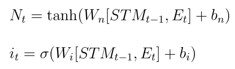
The Forget Gate
Forget gate takes LTM and multiplies it by a forget factor. Forget factor is an output of another small neural network, which takes the combination of STM and event, multiplies by weight, adds bias and runs through sigmoid. The equation for forget factor is below.
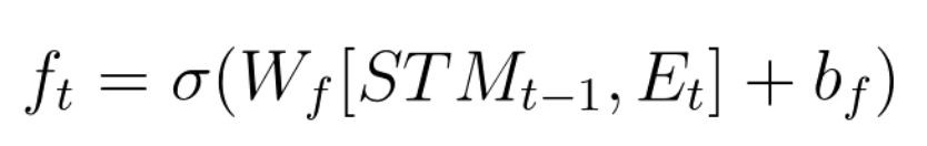
The Remember Gate
This one just adds the output of the learn gate and combines it with the output of the forget gate.
The Use Gate
Also called the output gate, this one takes the output of the forget and learn gates and combines them to obtain the new short term memory and the output (which are the same thing). The way it is done is the small neural network on top of forget gate with tanh function and another network on top of learn gate with sigmoid. The results are then multiplied to provide a new STM.
Overall architecture
The overall architecture is quite arbitrary and is the result of experimentation. It is proven to work, however may be changed and is not set in stone.
Other architectures which work well are Gated Recurrent Unit (GRU) [4]. It’s main difference from LSTM is that it has only one working memory, not LTM and STM. It does have two gates - update and combine.
Links:
Lesson 12: Implementing RNNs and LSTMs
RNNS have an intrinsic difficulty learning long-range interactions due to exploding/vanishing gradients. This happens because of multiple multiplications of the same number, so if the number is below 1 the product will eventually go to zero and if it is larger than 1 it will go to infinity.
Links:
- NaNoGenMo novel generation contest
- Karpathy’s implementation of RNN in PyTorch
- Implementation of LSTM in Tensorflow API
- Building RNN in TF from ground up
Lesson 13: Hyperparameters
No magic numbers that work everywhere. HP can be grouped in two categories. First is Optimizer hp, these will include learning rate, minibatch size, number of training iterations. Second is Model hp. These will include number of layers and some model-specific parameters related to architecture.
Learning rate is the single most important parameter. There are many different scenarios where we may be converging too slowly if rate is too small or even diverging if rate is too high. Some of these issues may be addressed by decaying learning rate. Also there are adaptive learning algorithms, like Adam and Adagrad.
Minibatch size is the second important hyperparameter. Historically there was a debate between using online (stochastic) training on each point one-by-one vs using the entire dataset. 32 is a good starting point. There is a computational boost benefit of using larger batch sizes, however using smaller batches actually introduces more noise, which allows to avoid algorithm stucking in a local minima. So, both big and small size have their benefits. According to paper too large batch sizes significantly decrease accuracy, so anywhere from 32 to 256 is a good range.
Early stopping with validation error helps to choose the best number of training iterations/epochs.
For the number of layers and hidden units - “in practice it is often the case that 3-layer neural networks will outperform 2-layer nets, but going even deeper (4,5,6-layer) rarely helps much more. This is in stark contrast to Convolutional Networks, where depth has been found to be an extremely important component for a good recognition system (e.g. on order of 10 learnable layers).” ~ Andrej Karpathy in https://cs231n.github.io/neural-networks-1/. Increasing the number of hidden units increases the capacity of model to learn, but increase it too much and you will likely overfit. It is recommended to have more hidden units than inputs.
For RNN architectures - there is no clear winner between LSTM and GRUs. Two layers are sufficient usually. Word embeddings sizes typically don’t go beyond 500 or 1000.
Links:
- Jay Alammar’s blog on NN visualisation
- Empirical Evaluation of Gated Recurrent Neural Networks on Sequence Modeling
- An Empirical Exploration of Recurrent Network Architectures
- Visualizing and Understanding Recurrent Networks
- https://colah.github.io/posts/2015-08-Understanding-LSTMs/
- Massive Exploration of Neural Machine Translation Architectures
- How to Generate a Good Word Embedding?
Lesson 14: Sentiment Analysis
Following deep-learning repo. Predict sentiment based on IMDB movie reviews.
Steps:
- Pre-process review and split into words
- Use embedding layers to convert words into embedding space (you can use Word2Vec or GloVe weights).
- Create training, test and validation sets
- Build the TF graph
- Train the network
Lesson 15: Project
Using LSTM for time-series prediction (Apple stock prices) and generation of text. There were 5 assignments, two were related to converting sequences into windowed X-y representations. Two were related to creating LSTM networks in Keras. One was related to cleaning up the text.
Links:
Lesson 16: Generative Adversarial Networks
Multiple applications in generating new images or doing image to image or text to image translations. Multiple examples in generating synthetic data for other ML or RL algorithms. Examples of using in scientific domain to compliment/replace physical measurements and simulations.
GANs consist of two NNs. First is the generator NN, which goal is to generate realistic looking images from random noise fed into it. It is trained by learning the probability distributions inherent in real images. Once it generates some images it is fed to a second NN, which is called “Discriminator”. It is just a regular classifier NN, which during the training process is constantly fed with real images and the ones generated by “Generator”, so D guides G towards producing more realistic images. “Police vs counterfeiters” analogy. Adversarial in GAN means exactly this - that the Generator and Discriminator networks are competing against each other.
For a case of MNIST hand-written digits generation the GAN architecture may we can have four layers total - two first ones form a G network (one hidden layer with output layer running tanh) and D network (one hidden layer and output with sigmoid to output probabilities). The training of GANs is different from usual NN is that they require two optimizations - one for D and one for G network. We also need to define two separate loss functions - g_loss and d_loss for both networks correspondingly.
Exercise is following the GAN example in Udacity DL lab.
Lesson 17: Deep Convolutional GANs (DCGAN)
Transposed convolution to go from narrow and deep layers to shallow and wide. Was proposed by the original DCGAN paper. In DCGAN there are no maxpool or dense layers - just convolutions. They also use batch normalization at each layer. Generator is responsible for upsampling noise to images. Discriminator by analogy is used to downsample images and similary does not use any maxpool or dense layers.
Batch norm is an important factor in making DCGAN work. Proposed in 2015 as a technique to accelerate deep network training. Essentially at every layer the input is normalized to have a mean of 0 and std of 1.
Links:
Lesson 18: Semisupervised Learning
Semisupervised learning using GAN to improve the performance of the classifier. Semi-supervised means that the model will be training both on the labeled data as well as on unlabeled data. When we use GANs to generate images the Generator is the main goal, while Discriminator is of secondary importance. In semi-supervised learning Discriminator is the goal.
To achieve we change the output of D to softmax having N real classes + 1 class for fake images. Training loss is then the combination of regular supervised cross-entropy for real examples with labels. For all other examples and for fake images we use the GAN cost. OpenAI have shown that this approach introduced 3x improvement over previous best semisupervised learning methods. It is still worse than supervised learning which, however, requires a lot of labeled data. Another way to look at it is that we place a regular classifier inside a GAN framework and feed it with three sources of data - first real images with labels to actually train classifier, second real images without labels, where discriminator just has to maximize the probability of all real classes and finally discriminator also needs to learn how to reject the fake images.
Overall semi-supervised learning with GANs is easier to achieve than a good image generation with GANs.
Links:
Lesson 20: Intro to Computer Vision
Some applications of CV:
- self-driving cars
- medical image and analysis
- photo tagging and face recognition
- image retrieval
- automatic image captioning
- emotions recognition (emotion AI)
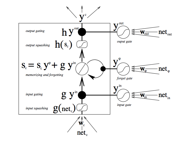
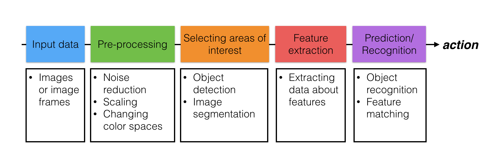
CV pipeline includes the following steps:
- input data
- image preprocessing
- selecting areas of interest
- feature extraction
- prediction/recognition
Links:
Lesson 21: Natural Language Processing
Some use cases of NLP:
- providing an augmented HMI allowing humans to communicate with machine with plain language (i.e. airbnb search case)
- NLP as a part of more complex AI systems involving vision
- Speech to text
- Tone analyzers and sentiment analysis
- Analyzing medical histories to bring up important facts (Watson)
- Sites -> apps -> bots
- One-to-one vs one-too-many interactions
Speech recognition industry record is 5.5% (2017-2018) vs human of 5.1%.
Artificial Narrow Intelligence (weak AI), e.g. Jeopardy Watson Artificial General Intelligence (strong AI or human AI), e.g. robot assistant Artificial Superintelligence, e.g. SkyNet, better than human at any field, aware of itself.
Some of Watson Cognitive APIs/use cases:
- spam detection
- FAQ bots
- Discovery and conversation services
- tone analysis
Links:
Lesson CV-4: Image Representation and Analysis
CV pipeline:
- Input data
- Pre-processing (noise reduction, scaling, changing color)
- Selecting areas of interest (object detection, image segmentation)
- Feature extraction (extracting data about features)
- Prediction/Recognition (object recognition, feature matching)
Pre-processing step
Typical techniques - changing color schemes, changing spatial representation and transforming, filters to sharpen or blur.
Pre-processing using pixel values
Grayscale typically is more useful for object recognition. Intensity can provide enough info for object detection. Color is important in some of the cases, like medical diagnostics, self-driving car detecting different lines, etc.
Blocking out one object works well when it stands out, e.g. chromakeying. But it does not work well when colors are changing or lighting conditions change, etc.
There are multiple 3D color space representations. We’ll be using HSV (Hue, Saturation, Value). HSV provides better separation of colors in different light conditions, gradients and minor color changes. Hue goes from 0 to 180 as degree.
Pre-processing using geometric transforms
Geometric transforms have multiple uses. One of the most common is transforming the text to align it properly prior to text recognition. OpenCV has functions to geometrically transform, say, skewed images and takes two vectors of coordinates - the original one and the one we’d like to transform it to.
import numpy as np
import matplotlib.pyplot as plt
import cv2

# Read in the image
image = cv2.imread('license_plate_skew.jpg')
# Convert to RGB (from BGR)
image = cv2.cvtColor(image, cv2.COLOR_BGR2RGB)
# ---------------------------------------------------------- #

## TODO: Define the geometric tranform function
## This function take in an image and returns a
## geometrically transformed image
def geo_tx(image):
    image_size = (image.shape[1], image.shape[0])

    ## TODO: Define the four source coordinates
    source_pts = np.float32(
        [[300, 800],
         [600, 810],
         [600, 1050],
         [300, 950]])

    ## TODO: Define the four destination coordinates
    ## Tip: These points should define a 400x200px rectangle
    warped_pts = np.float32(
        [[450, 800],
         [900, 800],
         [900, 1000],
         [450, 1000]])

    ## TODO: Compute the perspective transform, M
    M = cv2.getPerspectiveTransform(source_pts,warped_pts)

    ## TODO: Using M, create a warped image named `warped`
    warped = cv2.warpPerspective(image, M, image_size)

    return warped


# ---------------------------------------------------------- #
# Make a copy of the original image and warp it
warped_image = np.copy(image)
warped_image = geo_tx(warped_image)

# Visualize
f, (ax1, ax2) = plt.subplots(1, 2, figsize=(20,10))
ax1.set_title('Source image')
ax1.imshow(image)
ax2.set_title('Warped image')
ax2.imshow(warped_image)
Pre-processing using filters
High-pass filters detect the big changes in intensity and color. They are used to sharpen the image and to enhance high-frequency parts of an image. High-frequency in this case means a rapid change in color or intensity. High-pass filters emphasize big changes and create edges along those areas. High-pass filters are convolution kernels, e.g. 3x3 matrix of values or weights. The sum of elements should be equal to zero, if not - the whole processed image will be lightened or darkened. Edge detection, for instance looks at comparing the center pixel to it’s neighbours.
Convolution process means element-wise multiplication of kernel by a piece of image and summing all values to come up with a new value for a specific pixel considered (center value).
Different kernels are good for different purposes, e.g. identifying horizontal or vertical changes, identifying edges, etc.
Sobel filter is used for abrupt intensity changes in x and y directions. There are two variations - Sobel X and Sobel Y. Sobel X example is shown below.
OpenCV has a function to convolve an image with a provided kernel:
kernel = np.array([[ -1, -2, -1],
                   [ 0, 0, 0],
                   [ 1, 2, 1]])
filtered_image = cv2.filter2D(gs_image, -1, kernel)
High-pass filters often exaggerate noise in the images, which is not helpful. Low-pass filters can help with noise and is often applied to blur the image before the high-pass filter. Low-pass filters blur the image and block the high-frequency parts of the image.
The simplest example of a blur filter is an averaging filter:
Since we are summing the result of element-wise multiplication we are getting the average value of all 9 pixels. We need to normalize it by 1/9 to preserve the same overall intensity.
Gaussian blur is an improved version which preserves edges. It is one of the most used low-pass filters. It is quite similar to the first edge-detection filter, except all weights are positive and the result is normalized. The Gaussian blur is implemented as a function in OpenCV.
The edge detection workflow is the following:
- Convert image to grayscale
- Apply low-pass filter (Gaussian blur)
- Apply high-pass filter
- Apply binary threshold (convert to B&W) to emphasize edges
Canny edge detection is used widely in CV applications and implements the workflow above with some improvements to emphasized edges following the high-pass filter. It is available as a function in OpenCV as well. Note - it is recommended to use 1:2 or 1:3 ratios when defining threshold values for Canny function.
Lesson CV-4: Image Segmentation
Image segmentation is the process of dividing image in segment or unique areas of interest. It is done in two ways:
- By connecting a series of detected edges
- By grouping an image into separate regions by area or distinct trait (e.g. color)
Image contouring is a useful technique. OpenCV has a series of functions for contouring. Prior to using these it is beneficial to apply thresholding to emphasize boundaries and objects.
# Read in an image and convert to RGB
image = cv2.imread('thumbs_up_down.jpg')
image = cv2.cvtColor(image, cv2.COLOR_BGR2RGB)

# Convert to grayscale
gray = cv2.cvtColor(image,cv2.COLOR_RGB2GRAY)
# Create a binary thresholded image
retval, binary = cv2.threshold(gray, 225, 255, cv2.THRESH_BINARY_INV)

# Find contours from thresholded image
retval, contours, hierarchy = cv2.findContours(binary, cv2.RETR_TREE, cv2.CHAIN_APPROX_SIMPLE)
Hough transformation moves lines in image space to points in Hough space which is formed in (m, b) coordinates, where m is the slope and b is the intercept. Hough-based edge detection in OpenCV. Hough transform may be used in finding the road boundaries for self-driving cars.
K-mean clustering is used to form clusters based on some common traits. By choosing the right cluster number it is possible to mask different objects.
CNNs can be used for image segmentation as well, although there are not very computationally effective. The naive approach was to run multiple CNNs per each small piece of an image and predict whether there is any recognizable object inside that piece. There is an ongoing research work to improve the efficiency of CNNs for image detection. Mask R-CNN is the state-of-the-art algo as of 2017.
Links:
Lesson CV-6: Features and Object Recognition
The most important property of the feature in CV applications is the repeatability, i.e. whether it will be detected in two or more images of the same scene under different conditions.
Three categories of features:
- Edges
- Corners (intersection of edges)
- Blobs (region based features)
Corners are the most repeatable features due to their uniqueness on a given image. Corner detection algorithm is looking for big variations in the direction and magnitude of gradients. Corner gradient in openCV.
Dilation and erosion are known as morphological operations. They are often performed on binary images, similar to contour detection. Dilation enlarges bright, white areas in an image by adding pixels to the perceived boundaries of objects in that image. Erosion does the opposite: it removes pixels along object boundaries and shrinks the size of objects.
As mentioned, above, these operations are often combined for desired results! One such combination is called opening, which is erosion followed by dilation. This is useful in noise reduction in which erosion first gets rid of noise (and shrinks the object) then dilation enlarges the object again, but the noise will have disappeared from the previous erosion!
Closing is the reverse combination of opening; it’s dilation followed by erosion, which is useful in closing small holes or dark areas within an object. Closing is reverse of Opening, Dilation followed by Erosion. It is useful in closing small holes inside the foreground objects, or small black points on the object.
Example of corner detection script:
image = cv2.imread('waffles.jpg')
image = cv2.cvtColor(image, cv2.COLOR_BGR2RGB)
# ---------------------------------------------------------- #

def corner_detect(image):
    gray = cv2.cvtColor(image, cv2.COLOR_RGB2GRAY)
    gray = np.float32(gray)
    corners = cv2.cornerHarris(gray,2,3,0.04)
    corners = cv2.dilate(corners,None)
    return corners

corners = corner_detect(image)
threshold = 0.3*corners.max()

# ---------------------------------------------------------- #
if(corners is not None):
    corner_image = np.copy(image)

    # Iterate through all the corners and draw them on the image (if they pass the threshold)
    for j in range(0, corners.shape[0]):
        for i in range(0, corners.shape[1]):
            if(corners[j,i] > threshold):
                # image, center pt, radius, color, thickness
                cv2.circle(corner_image, (i, j), 1, (0,255,0), 1)

    # Plot the result
    f, (ax1, ax2) = plt.subplots(1, 2, figsize=(20, 10))
    f.tight_layout()
    ax1.imshow(corners, cmap='gray')
    ax1.set_title('Dilated Corners')
    ax2.imshow(corner_image, cmap='gray')
    ax2.set_title('Thresholded Corners')
Histogram of Oriented Gradients
It is possible to construct a vector of features, by estimating the edges on the image. Then split the image into cell and within each cell calculate the direction of the gradient for the edge. This matrix of gradient directions may then be flattened and used as a feature vector.
HOG is one of the examples of algorithms using the above-described principle. It comprises of the following steps:
- Calculate the magnitude and direction of the gradients in the image at each pixel (using Sobel filters)
- Groups pixels into square cells
- Count how many gradients in each cell fall into specific range of orientations
The result is the vector of features, which can be used in classifier to detect similar objects. The main assumption underneath is that HOG features will be unique to a specific object, wherever/however it appears.
HOG has a function in openCV:
# Parameters you define for a HOG feature vector
win_size = (64, 64)
block_size = (16, 16)
block_stride = (5, 5)
cell_size = (8, 8)
n_bins = 9

# Create the HOG descriptor
hog = cv2.HOGDescriptor(win_size, block_size, block_stride, cell_size, n_bins)

# Using the descriptor, calculate the feature vector of an image
feature_vector = hog.compute(image)
SVM has been shown to work well with HOG and is quite fast compared to CNNs obviously.
Haar Cascades
Haar features are quite similar to convolution layers, but done at a larger scale. They can detect features like lines, rectangles and more complex features. After feature detection Haar algorithm applies a cascade of classifiers to reject parts of the images which are not classified as the face. As a result it focuses on processing and recognizing only related parts of the image. By rejecting parts of the image Haar cascade is a very fast algorithm which can be applied to a video stream on a laptop computer.
Haar cascade may be trained to recognize objects other than face - see openCV documentation.
Links:
Motion
Optical flow is one of the techniques to analyze motion on video streams. It is based on few assumptions:
- Pixel intensities stay consistent between frames
- Neighboring pixels have similar motion
Optical flow is then tracks a point to understand the speed of movement and also predict the future positions of the object.
To perform optical flow on a video or series of images, we’ll first have to identify a set of feature points to track. We can use a Harris corner detector or other feature detector to get these. Then, at each time step or video frame, we track those points using optical flow. OpenCV provides the function calcOpticalFlowPyrLK() for this purpose; it takes in three parameters: previous frame, previous feature points, and the next frame. And using only this knowledge, returns the predicted next points in the future frame. In this way, we can track any moving object and determine how fast it’s going and where it’s likely to move next!