WEKA classification
There was a question posted on stackoverflow on classification issues in WEKA. The datasets are available via web-archive. Since *.csv files were not available I downloaded *.ARFF and converted them to *.csv manually, as the format appeared to be quite simple. This is the list of features available to be placed in first row to construct the dataframe with column names.
duration,protocol_type,service ,flag,src_bytes,dst_bytes,land,wrong_fragment,urgent,hot,num_failed_logins,logged_in,num_compromised,root_shell,su_attempted,num_root,num_file_creations,num_shells,num_access_files,num_outbound_cmds,is_host_login,is_guest_login,count,srv_count,serror_rate,srv_serror_rate,rerror_rate,srv_rerror_rate,same_srv_rate,diff_srv_rate,srv_diff_host_rate,dst_host_count,dst_host_srv_count,dst_host_same_srv_rate,dst_host_diff_srv_rate,dst_host_same_src_port_rate,dst_host_srv_diff_host_rate,dst_host_serror_rate,dst_host_srv_serror_rate,dst_host_rerror_rate,dst_host_srv_rerror_rate,classI read both training and test datasets into pandas DataFrame. Merge them into one to do the feature processing and later split using the original ratio. Three features which had strings as values were factorized, as well as the outcome variable “class”.
The code is below. Libraries used are numpy, pandas, scikit-learn and matplotlib. One can use Anaconda python distribution which has these preinstalled. The code contains portions posted on scikit-learn site, namely the learning curve and confusion matrix plotting routines.
import pandas as pd
import numpy as np
import matplotlib.pyplot as plt
from sklearn import metrics
from sklearn import ensemble
from sklearn import learning_curve
from sklearn import cross_validation
pd.options.mode.chained_assignment = None #suppress chained assignment warning
#random forest classifier
#input - X and y
#output
def RandomForest(X,y,n_est,factors):
#-------------------------------------------
#Random forest classifier
forest = ensemble.RandomForestClassifier(oob_score=True,
n_estimators=n_est)
forest.fit(X,y)
#-------------------------------------------
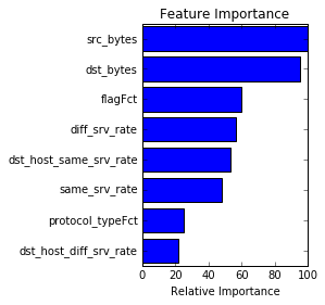
#feature importance
feat_impo = forest.feature_importances_
feat_impo = 100.0*(feat_impo / feat_impo.max())
feat_list = X.columns.values
fi_threshold = 20
important_idx = np.where(feat_impo > fi_threshold)[0]
#Create a list of all the feature names above the importance threshold
important_features = feat_list[important_idx]
#Get the sorted indexes of important features
sorted_idx = np.argsort(feat_impo[important_idx])[::-1]
pos = np.arange(sorted_idx.shape[0]) + .5
plt.subplot(1, 2, 2)
plt.barh(pos, feat_impo[important_idx][sorted_idx[::-1]], align='center')
plt.yticks(pos, important_features[sorted_idx[::-1]])
plt.xlabel('Relative Importance')
plt.title('Feature Importance')
plt.draw()
plt.show()
return forest
#source - sklearn
#http://scikit-learn.org
#/stable/auto_examples/model_selection/plot_learning_curve.html
def plot_learning_curve(estimator, title, X, y, n_jobs=1):
train_sizes=np.linspace(0.1, 1.0, 10)
plt.figure()
plt.title(title)
plt.xlabel("Training examples")
plt.ylabel("Score")
plt.ylim([0,1.2])
train_sizes, train_scores, test_scores = learning_curve.learning_curve(
estimator, X, y, cv=10, n_jobs=n_jobs, train_sizes=train_sizes)
train_scores_mean = np.mean(train_scores, axis=1)
train_scores_std = np.std(train_scores, axis=1)
test_scores_mean = np.mean(test_scores, axis=1)
test_scores_std = np.std(test_scores, axis=1)
plt.grid()
plt.fill_between(train_sizes, train_scores_mean - train_scores_std,
train_scores_mean + train_scores_std, alpha=0.1,
color="r")
plt.fill_between(train_sizes, test_scores_mean - test_scores_std,
test_scores_mean + test_scores_std, alpha=0.1, color="g")
plt.plot(train_sizes, train_scores_mean, 'o-', color="r",
label="Training score")
plt.plot(train_sizes, test_scores_mean, 'o-', color="g",
label="Cross-validation score")
plt.legend(loc=1)
return plt
#source - sklearn
#http://scikit-learn.org
#/stable/auto_examples/model_selection/plot_confusion_matrix.html
def plot_confusion_matrix(cm, factors, title='Confusion matrix',
cmap=plt.cm.Blues):
plt.imshow(cm, interpolation='nearest', cmap=cmap)
plt.title(title)
plt.colorbar()
tick_marks = np.arange(2)
plt.xticks(tick_marks, factors, rotation=45)
plt.yticks(tick_marks, factors)
plt.tight_layout()
plt.ylabel('True label')
plt.xlabel('Predicted label')
if __name__ == '__main__':
#read dataset
train = pd.read_csv(open('KDDTrain+.csv', 'rb'),sep=',')
test = pd.read_csv(open('KDDTest+.csv','rb'),sep=',')
full = pd.concat([train,test])
#factorizing features with labels
full['protocol_typeFct'] = full.protocol_type.factorize()[0]
full['serviceFct'] = full['service '].factorize()[0]
full['flagFct'] = full.flag.factorize()[0]
[full['result'],factors] = full['class'].factorize()
full = full.drop(['protocol_type','service ','flag','class'],axis=1)
#selecting X and y datasets
X = full.loc[:,'duration':'flagFct']
y = full.result
#split dataset in training and test following the original order
X_train = X[:125973]
y_train = y[:125973]
X_test = X[125973:]
y_test = y[125973:]
# X_train, X_test, y_train, y_test = cross_validation.train_test_split(
# X, y, test_size=0.25, random_state=1337)
#Random forest
n_estimators = 50
title = 'Random Forest: '+str(n_estimators)+ \
' est. and '+str(X.shape[1])+' feat.'
forest = RandomForest(X_train, y_train, n_estimators, factors)
plot_learning_curve(forest, title, X_train, y_train, n_jobs=1)
#prediction and evaluation
y_pred = forest.predict(X_test)
#-------------------------------------------
#Compute confusion matrix
cm = metrics.confusion_matrix(y_test, y_pred)
title = 'Confusion matrix: '+str(n_estimators)+ \
' est. and '+str(X.shape[1])+' feat.'
plt.figure()
plot_confusion_matrix(cm,factors,title)
#-------------------------------------------
#-------------------------------------------
#Evaluation report
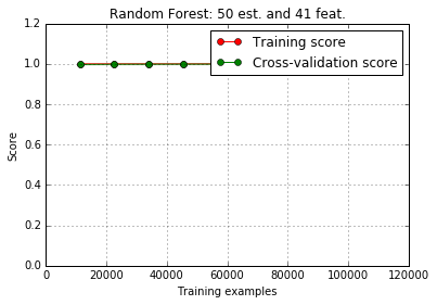
print metrics.classification_report(y_test,y_pred,target_names = factors)Script provides three plots. First is the feature importance. Second is the learning curve which looks somewhat weird as both training and cross-validation scores are perfect. After delving deeper into dataset it looks like the original website hosting the dataset mentions that it had too many repeat values, which could explain these scores.
Finally the confusion matrix for the test dataset. The precision drops to 65% for “normal” case and recall is high. Perhaps adjusting the threshold values for classifier will help.
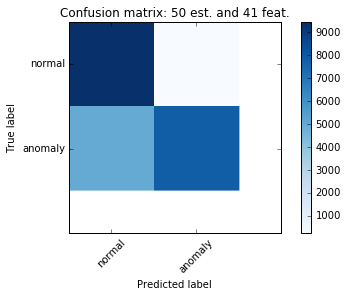
The final fit report is below as well:
             precision    recall  f1-score   support

     normal       0.65      0.97      0.78      9711
    anomaly       0.97      0.61      0.75     12833

avg / total       0.83      0.77      0.76     22544
Overall the performance of the classifier on the test set is consistent with the one mentioned in the original question on stackoverflow.